Lesson 5: Models of Learning
In this and the coming decades, climate change will alter the frequency and severity of the environmental hazards the threaten human life and livelihoods in communities all over the globe. Cities close to the equator will face more frequent and severe bouts of life-threateningly high temperatures. Coastal communities will experience rising sea levels and more powerful cyclones and hurricanes. Communities that thrive on agriculture, fishing and forestry will experience the dying off of plant and animal species on which their economies rely. Cities in arid regions will encounter greater volatility in rain and snowfall.
How much human suffering and loss these changes wreak depends to a substantial extent on how much governments do in the coming years to facilitate human resilience to natural hazards. The populations of coastal regions, for instance, will suffer less if their governments adopt regulations that prevent the destruction of wetlands that dampen storm surges, while populations of cities at risk of heat waves can be protected by government investments in tree cover and public cooling facilities.
What do you know at this point about the environmental hazards that will threaten the places you call home in the coming decades? What do you know about the investments governments are making in those places to mitigate those hazards? How likely do you think it is that governments will make the investments and other changes required to adapt to our changing climate?
Many of us are aware that our welfare and that of our loved ones depends on governments adopting policies and making investments that mitigate natural hazards. But almost none of us are in a position to know the specific details of the policies and investments our governments are or are not making. And even fewer have the expertise to determine exactly what government policies and investments are appropriate in light of the specific hazards facing any given place or region. These details will only be known, if at all, by the tiny portion of persons whose full-time jobs involve making, researching or reporting on government policy. The rest of us will be left to judge the performance of our governments based on what we see, hear and read in the media.
Most of us face, then, what political scientists call a problem of political accountability. Although we each rely on governments to act in our interest, we have only a sliver of the information or knowledge we would need to know for sure whether any given government has acted or is acting as such. At best, we can use the partial information we glean from media reports and our day-to-day experiences to make inferences (which will, inevitably, be incorrect) about whether our political leaders have acted responsibly, and use what little political power we have to reward or punish them accordingly.
In PPT, we used models of learning to depict the process through which political actors use limited information to update their beliefs about critical facts that they cannot ascertain with certainty. In this lesson, you’ll learn gain some familiarity with how models of learning work.
An Example
Think once again of the imaginary city sitting on the riverbank that we introduced in Lesson 4. Imagine a resident of that city who, at a given moment in time, is uncertain about whether the city’s mayor made investments in the city’s flood control infrastructure that are in that resident’s best interest.
Suppose this resident, like most of us, has no ability to directly observe the details of her political representatives’ behavior in office. And suppose that the resident, like most of us, lacks the expertise to evaluate any particular action by a politician (such as spending a particular sum on a particular project) that she happens to observe. On what basis can she judge whether the mayor has in fact acted in her interest?
Let’s consider the possibility that the resident’s personal experiences, which she can directly observe and evaluate, might allow her to make imperfect inferences about the mayor’s behavior. The resident cannot spend all day in City Hall watching every move the mayor makes. And even if she did, she isn’t a hydrological engineer, and so couldn’t tell you what exactly the mayor ought to do with the funds he has available to spend on flood control. But when a storm hits the city, the resident will know whether or not flood waters damage her home. Picture her standing in her kitchen the day after a storm. She won’t know exactly what the mayor did with her tax money. She won’t know whether whatever the mayor did with that money was the right thing for her. But she will know whether or not she, standing in her kitchen, is knee-deep in water. And presumably, whether she is knee-deep in water is an imperfect indicator of whether the mayor acted in her interest – i.e. it is less likely that the mayor acted in her interest if she is knee-deep in water, and more likely otherwise.
To depict these ideas, imagine a moment sometime before a storm hits the city. Suppose at the moment that resident is uncertain about two things:
- whether the mayor has made investments in flood control infrastructure that are in the resident’s interest.
- whether the next storm that hits the city will cause flooding that damages her home.
We’ll model the resident’s marginal uncertainty about (a) and uncertainty about (b) conditional on (a) using a Marginal-Conditional Diagram like this:

There are two choices we’ve made in building this model that it’s critical to notice.
First, we’ve assumed that the resident’s home is more likely to be damaged if the mayor has not acted in the resident’s best interest than if the mayor has acted in the resident’s best interest. Thus flood damage to the resident’s home (which the resident can observe and evaluate directly) is to some extent informative about the mayor’s behavior (which the resident cannot observe and evaluate directly). Specifically, we’ve set: P \left( \text{resident's home damaged} | \text{mayor did not act in resident's interest} \right) = \frac{96}{100} and P \left( \text{resident's home damaged} | \text{mayor acted in resident's interest} \right) = \frac{92}{100}
Second, we have not assumed that the resident will ever have the ability to know with certainty whether the mayor has acted in her interest. In the model as we’ve specified it, the resident’s home has some chance of being damaged and some chance of not being damaged regardless of the mayor’s behavior. Further, the mayor’s behavior has only a slight effect on the relative likelihood that the resident’s home is damaged – causing the likelihood of damage to vary between \frac{2}{100} and \frac{4}{100}. So the effects of the storm that the resident can directly observe cannot amount to definitive evidence about the mayor’s performance. Thus the model tries to capture the fact that direct experience can reduce but not eliminate ordinary persons’ uncertainty about whether politicians are acting in their interests. It does this by depicting a situation in which the resident’s direct experience can tell her something about the mayor’s performance, but can never fully resolve her uncertainty.
To use this model to depict how the resident might learn about the mayor’s behavior, imagine a storm hits the city, and thus the resident directly observes whether her home is damaged by flooding. In this event, her uncertainty is partially resolved. After the storm has passed, she knows whether flooding caused by the storm has damaged her home. But she remains uncertain about the mayor’s behavior. It looks like this:
There are two important features of models of learning that this diagram illustrates. First, models of learning depict change in beliefs over time. More precisely, the model depicts the resident’s beliefs at two distinct moments: before the storm (on the left) and after the storm (on the right). All models of learning have this basic structure. Thus we use the general term prior beliefs to refer to the uncertainty depicted before the learning event, and the term posterior beliefs to refer to the uncertainty depicted after the learning event, like this:

Second, posterior beliefs in a model of learning are simply conditional beliefs. Consider, for instance, the resident’s uncertainty about whether the mayor has acted in her interest after the storm has passed and she has seen that her home was not damaged by flooding. This uncertainty is simply the uncertainty about the mayor’s behavior conditional on the knowledge that her home was not damaged by the storm. Thus, when we specify prior beliefs using a Marginal-Conditional Diagram as we have in this example, we can use the techniques for calculating probabilities with Marginal-Conditional Diagrams taught in Lesson 4 to derive posterior beliefs.
For instance, suppose the storm does not damage the resident’s home. To calculate the probability assigned by the resident’s posterior beliefs to the event that the mayor acted in her interest, we first would gray out the portions of the diagram representing events in which the storm damaged the resident’s home, like this…

…Then we’d compute the portion of the remaining un-shaded part of the diagram representing the event that the mayor acted in the resident’s interests, like this:
Similarly, we could compute the probability assigned to the event that the mayor did not act in the resident’s interests in the resident’s posterior belief when her home was damaged like this:

Before moving on to more complex analyses, it’s worth taking a moment to make sure you see that events affect beliefs in this model in the direction you would expect. Specifically, recall a key assumption we made in building the model: The resident’s home is more likely to be damaged by the storm if the mayor has not acted in the resident’s interest than if the mayor has acted in the resident’s interest. Given that assumption, you should expect that the resident’s posterior belief will put higher probability on the event that the mayor acted in her interest when her home is not damaged than when her home is damaged.
Does this expectation bear out? If you calculate the probability that the mayor acted in the resident’s interests according to her posterior beliefs under each possible event (using the methods illustrated in the previous diagrams), you get the following: P\left( \left. \begin{array}{c} \text{mayor acted in} \\ \text{resident's interest} \end{array} \right| \begin{array}{c} \text{home} \\ \text{damaged} \end{array} \right) = \frac{3}{5} P\left( \left. \begin{array}{c} \text{mayor acted in} \\ \text{resident's interest} \end{array} \right| \begin{array}{c} \text{home not} \\ \text{damaged} \end{array} \right) = \frac{294}{390} If you find a common denominator so that you can compare these fractions, you’ll see that the former is smaller than the latter. It looks like this:
This figure shows a number line, ranging from 0 on the left to 1 on the right – i.e. it shows the range of possible values of any probability. It then marks three probabilities on the number line:
- The green dot marks the probability that the mayor has acted in the resident’s interest according to the resident’s prior belief – i.e. before the storm hits the city.
- The yellow dot marks the probability that the mayor has acted in the resident’s interest according to her posterior belief when her home has been damaged by the storm.
- The blue dot marks the probability that the mayor has acted in the resident’s interest according to her posterior belief when her home has not been damaged by the storm.
Notice how the direction in which the resident’s beliefs shift away from her prior belief (the green dot) depends on what she observes as a result of the storm. When the storm damages her home, the probability she puts on the mayor acting in her interest (the yellow dot) drops substantially. When the storm does not damage her home, the probability she puts on the mayor not acting in her interest (blue dot) increases slightly.
Pause and complete check of understanding 1 now!
Pause and complete check of understanding 2 now!
Pause and complete check of understanding 3 now!
Parameterized Models of Learning
Once again, think of the resident of the coastal city who cannot observe whether the mayor has made investments in flood control infrastructure that are in the resident’s interest, but can observe whether or not the next storm that hits the city results in flooding that damages her home. The model we built in the previous section sketches the idea that the resident can learn something about the mayor’s actions from the damage caused by the next storm. But it doesn’t allow us to explore the idea that how much the resident can learn might vary from one circumstance to another.
Consider, for example, the flood control infrastructure protecting New Orleans from coastal storms. Almost all of that infrastructure is owned and maintained by the U.S. Army Corps of Engineers, which is an agency of the U.S. Federal Government. As a local official elected by city voters, the Mayor of the City of New Orleans has no formal authority over how the Corps spends its money. After all, The Corps of Engineers is a federal agency, and thus answers solely to the U.S. Congress. To be sure, the Mayor has much more influence over the Corps than the typical resident of the city. As the city’s highest elected official, and a professional politician typically well-connected in Louisiana politics, the Mayor has pull with the U.S. Senators and House members representing Louisiana and the New Orleans area in Washington, DC. But, at best, this makes the Mayor of New Orleans no more than an especially well-connected lobbyist when it comes to influencing the city’s flood-control infrastructure.
How might the mayor’s limited influence affect what a resident of the city can learn about the Mayor’s performance from the damage that a coastal storm causes? More generally, how might the level of influence over infrastructure that any mayor enjoys affect what their constituents can learn from the performance of that infrastructure?
To explore these questions, we’ll elaborate the model we explored in the previous section somewhat. We’ll continue to assume that the marginal probability that the mayor uses his power (limited as it is) in the resident’s interest is \frac{3}{4}, and the marginal probability the mayor does not use his power in the resident’s interest is \frac{1}{4}. Further, we’ll maintain the assumption that conditional on the event that the mayor does not act in the resident’s interest, the probability that the resident’s home is damaged in the next storm is \frac{4}{100}. However, we’ll change the probability that the resident’s home is damaged conditional on the event that the mayor acts in the resident’s interest. Specifically, we’ll assume that this conditional probability is given by \delta \frac{4}{100}, where \delta is a parameter that we assume lies between 0 and 1. It looks like this:
This is a parameterized model of learning. It uses a parameter – in this case the Greek letter \delta (pronounced “del-tah”) – to help us to explore how changes in the model affect its behavior. For instance, suppose that the number for which the parameter \delta stands is very close to 1. Perhaps, for instance, \delta = \frac{99}{100}. At this value for \delta, the model looks like this:
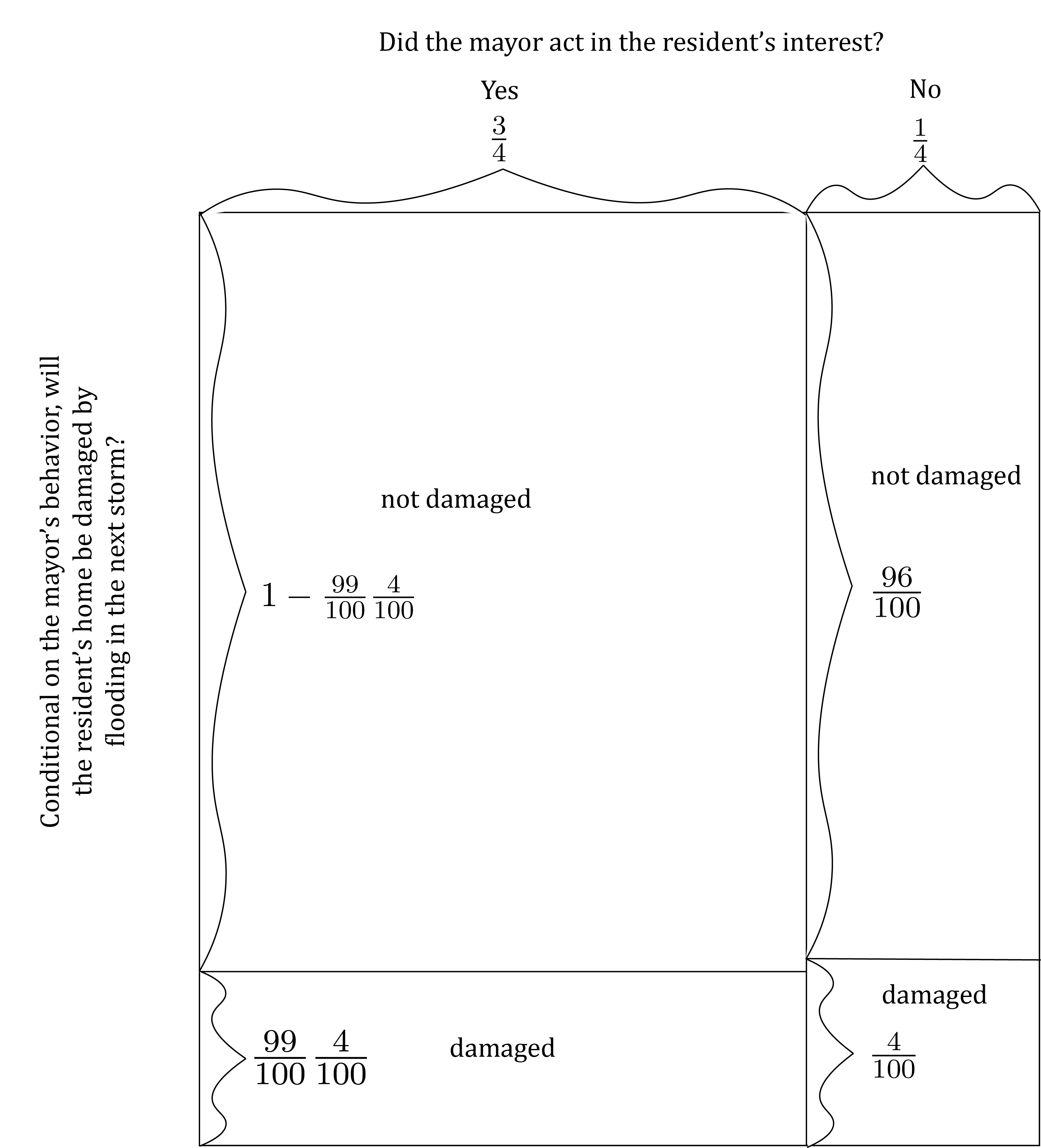
We can think of this as depicting a situation in which the mayor has only a tiny amount of influence over the city’s infrastructure, since in this case whether the mayor acts in the resident’s interest causes only a miniscule change in the probability that the resident’s home will be damaged.
In contrast, what happens if we set \delta to a number close to 0, as in \delta = \frac{1}{100}? At that value for \delta, the model looks like this…
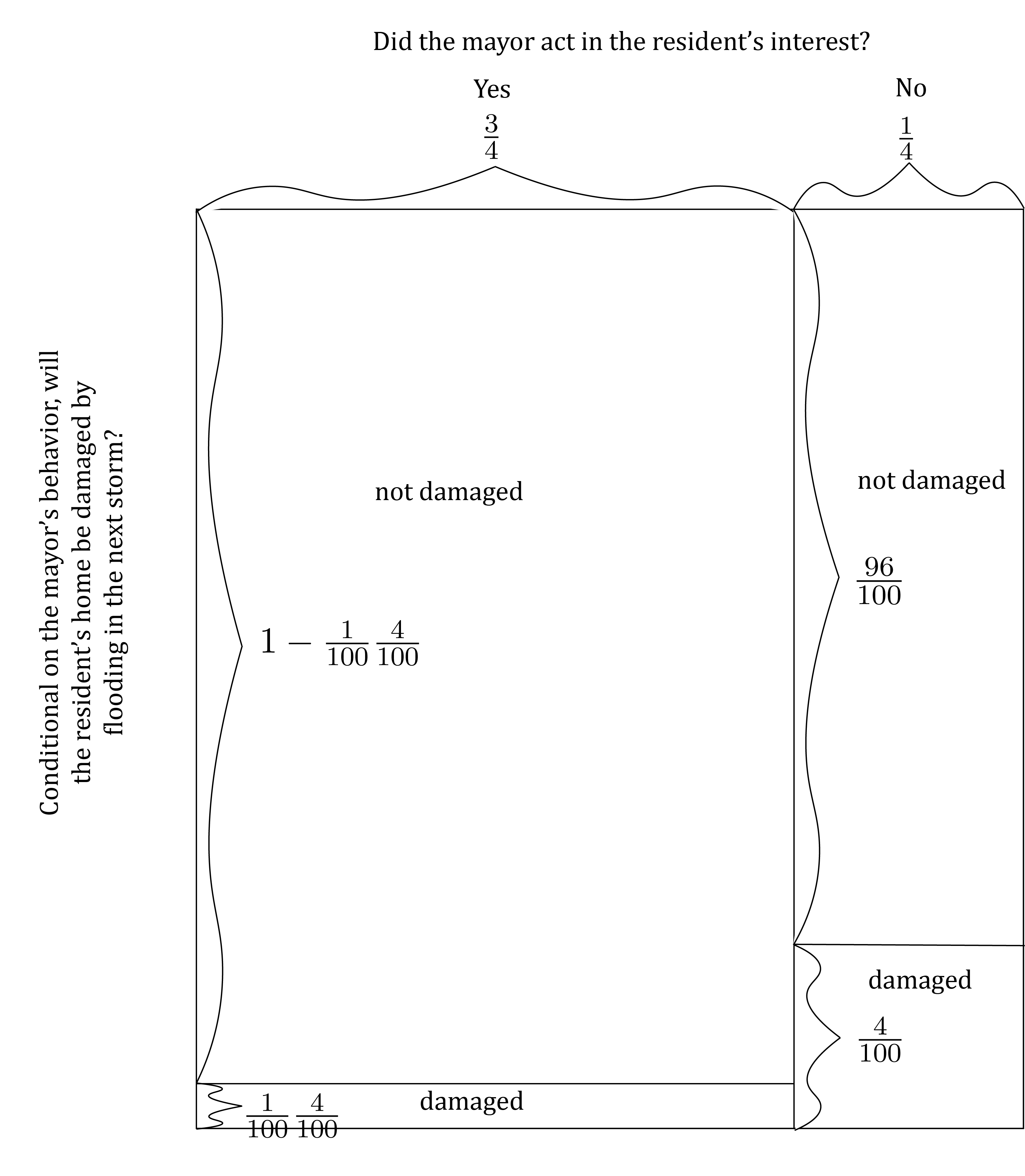
…depicting a situation where the mayor’s behavior can cause a very large change in the likelihood that the resident’s home will be damaged.
The overall goal of any parameterized model is to depict how changes in underlying conditions can change outcomes. In parameterized models of learning, we typically use parameters to show how the amount of information that is learned from an event can change from one circumstance to another.
We can explore the effects of the changes in the model here by first deriving the expressions describing the resident’s posterior beliefs as functions of the parameter \delta, like this:

We can then graph these posterior probabilities to get a sense of how they vary as \delta ranges from it’s minimum 0 to its maximum 1, like this:
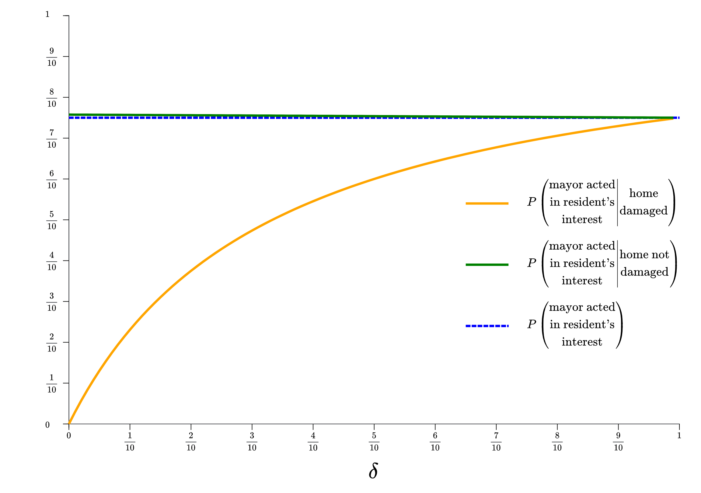
Make sure you understand each element of what this graph shows. First notice that horizontal axis shows the range of possible values of the parameter \delta, from 0 on the left to 1 on the right. Now take a look at the dotted blue line running across the graph. This is the probability that the mayor acts in the resident’s interest according to the resident’s prior belief. Recall, the model assumes that this probability is \frac{3}{4}, and thus you can see that the line intersects the vertical axis of the graph at \frac{3}{4}. The dotted blue line is essential for interpreting the graph. It depicts what the resident would believe about the mayor in the absence of any additional information. Thus you can think of that line as establishing the starting point from which any learning about the mayor would take place.
Now consider the orange curve, which arcs up from the bottom of the vertical axis at \delta = 0 and eventually meets the level of the prior belief (\frac{3}{4}) at \delta = 1. This is the probability that the mayor acted in the resident’s interest according to the resident’s posterior belief when the next storm damages her home. We’ve constructed that line by taking the expression for that posterior probability that we derived above… P \left(\left. \begin{array}{c} \text{mayor acted in}\\ \text{resident's interest} \end{array} \right| \text{home damaged} \right) = \frac{3\delta}{3\delta + 1} …and working out it’s shape as \delta ranges from 0 to 1. Notice two things about the orange curve. First, it lies below the probability that the mayor acted in the resident’s interest according to the resident’s prior belief (the dotted blue line) for all values of \delta. If you think about how the model works, you can make sense of this. After all, regardless of the value of \delta, the resident will always lose some faith in the mayor if her home is damaged. Thus the probability she assigns to the mayor acting in her interest will always go down (relative to where it started before the storm) in that event. Second, the the extent to which this probability is below the probability assigned by the prior belief varies with \delta. Specifically, the gap is very large when \delta = 0 and shrinks to nothing as \delta approaches 1. Make sense of this by looking again at the original specification of the model…
…and notice that \delta varies inversely with the extent to which the mayor’s behavior affects the probability that the resident’s home is damaged. As such, when \delta is close to 0, the mayor’s behavior has a large effect on the probability that the resident’s home is damaged. As a result, damage to the resident’s home causes a large change in the resident’s beliefs. In contrast, when \delta is close to 1, the mayor’s behavior has very little effect on the probability that the resident’s home is damaged, and thus damage to the resident’s home causes only a small change in her beliefs.
You can see a similar, although much less dramatic, pattern by inspecting the green curve, which shows the probability that the mayor acted in the resident’s interest according to the resident’s posterior beliefs when her home is not damaged. This line is farthest from the resident’s prior belief when \delta = 0, and gets closer to that prior belief as \delta increases.
Pause and complete check of understanding 4 now!