Lesson 4: Probabilistic Models of Uncertainty
Politics Under Uncertainty
On August 29, 2005, Hurricane Katrina made landfall in southern Louisiana and rapidly moved northward, passing over the area around the New Orleans. The tidal surge caused by Katrina overwhelmed the levees and floodwalls meant to protect the city and a catastrophic flood ensued. The exact number that died will never be known. About seven hundred persons were drowned during the night of August 29 and hundreds more died from lack of water, shelter and medical care in the days following the storm. Deaths and permanent displacements caused by the storm were concentrated among the area’s poor, and seemed to reveal an inability or unwillingness on the part of the city, state and federal governments to provide basic physical security for their citizens.
Either of two paths of thought might occur to you as you consider the Katrina disaster. One is retrospective: What caused all those people to die and be displaced in August of 2005? Who or what is to blame? What decisions were made prior to or during the storm that, if made differently, might have averted so much loss?
Another is prospective: Having learned from Katrina that a hurricane passing near New Orleans can cause catastrophe, what can be done that might protect the city and its residents from future storms? What would such measures cost and who should pay? Can those things be done, or must we just wait helplessly and watch it happen again?
In practice, these two directions of thought are not quite as distinct as they might at first seem. To see why, check out this image:
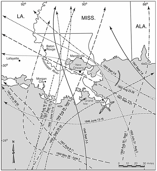
This shows the paths of all the hurricanes that passed through the region around New Orleans during the fifteen year period from 1945 through 1960. There’s nothing special about that particular range of dates. In just happens that the U.S. Government made a visualization of the paths of hurricanes over that fifteen year period, and that visualization is an extraordinarily vivid depiction of an essential fact about New Orleans: Hurricanes regularly and frequently threaten the city. If you created a similar graphic spanning any fifteen year period in the city’s history you would see a similar thick tangle of storms, with between one and three storms passing near the city every year, and one or two storms passing directly over the city every fifteen years.
So Katrina, terrible as it was, was not seen by longtime residents of New Orleans either as unprecedented or even unexpected. In fact, floods caused both by hurricanes and inland storms occur in the city almost every year. Sometimes the water causes no more than minor damage to a handful of properties. Other times several inches of water flood many blocks, causing millions of dollars in damage, and at most a few injuries or deaths. Rarely, but predictably (between once and twice every hundred years), a catastrophic flood like the one caused by Katrina occurs.
So, if we think retrospectively and ask “who is responsible for the death and destruction in New Orleans in 2005?”, any answer must hinge on what we know or suppose about the prospective thinking of residents of New Orleans and their political representatives in the years before 2005. They knew the city and region well. Just by living there – by experiencing floods throughout their lives and hearing stories of past floods handed down by their elders – they knew that hurricanes and other flood hazards were frequent, and in particular that monstrous storms were rare but always possible. Indeed, a hurricane nearly as destructive as Katrina inundated the city and killed hundreds of residents as recently as 1965. So the prospective question “what should we do to protect ourselves from the next storm”, has always been on the agenda in New Orleans. Whatever it was that turned Katrina into a catastrophe, then, stems from the politics resulting from that prospective question, asked every day of every year in the decades leading up to Katrina. Politics in each of those years at the local, state and federal levels culminated in choices by politicians to build sufficiently robust levees and other flood control infrastructure, or not; To permit and subsidize the construction of homes in flood-prone areas, or not; To destroy wetlands that if left in tact would dampen storm surges, or not; To prepare and fund adequate evacuation plans, or not.
Evidently, those politics did not produce policies and investments adequate to protect New Orleans residents and their homes from a storm the size of Katrina. In a series of decisions made throughout the 20th century, politicians at the local, state and federal level permitted the construction of thousands of homes on low-lying and sinking ground, drained and dredged swamps, marshes and wetlands that would have absorbed much of Katrina’s storm surge, built a system of levees and floodwalls too fragile to withstand a storm of Katrina’s size, and failed to plan and fund an evacuation program adequate to move the tens of thousands of New Orleans residents too poor to own personal vehicles out of harm’s way. Katrina, it turns out, is more aptly called a political disaster than a natural one. It amounted to a failure of political institutions to produce the investments required to protect persons from a natural hazard that, although irregularly occurring, was certain to occur at some point.
Can we hope for better? As climate change brings a surge of increasingly frequent and severe, and irregular but certain-to-occur natural hazards – floods, droughts, wildfires, extreme heat etc. – will our politics produce the public investments required to protect our lives and homes?
In this and the next two lessons, you’ll learn a set of tools political scientists use for modeling the politics of decisions like these – i.e. decisions made under uncertainty. At any given time, no one can know for sure when or where the next major natural hazard will occur or how severe it will be. Thus when governments make investments meant to protect persons from natural hazards like hurricanes, earthquakes and forest fires, the benefits of those investments are always uncertain. When politicians, say, raise taxes to fund seawalls that would divert storm surges away from populated areas, or burden landlords with building standards that require structures to be hardened to earthquakes, or fund controlled burns that inconvenience residents in the short run but lessen the chances of uncontrollable wildfires in the long run, no one can know for sure who will benefit, when, or how much.
This and the next two lessons teach two tools for modeling decisions under uncertainty: Probabilistic models of uncertainty and expected utility. These tools have applications far beyond the politics of natural hazards. Uncertainty is, after all, present in every aspect of life. But throughout we’ll use examples of natural hazards and the political decisions that can mitigate or exacerbate their effects to illustrate the concepts and techniques.
Probabilistic Models of Uncertainty: An Example
Imagine a city that sits on the banks of a river, just inland from where the river empties into the sea. Any such city can flood when a hurricane or cyclone comes ashore nearby, as the storm’s winds and low atmospheric pressure pull water from the sea up the river, and dump torrential rains into the river’s watershed. Imagine this city has experienced many coastal storms over the years, and scores of resulting floods. Most of these floods were small and caused no more than inconvenience. Some have been large but limited, damaging much property but harming no one. Two or three of the floods in the city’s recorded history have been catastrophic – killing hundreds and levelling whole neighborhoods.
Imagine this city has a new mayor. This mayor, rather than just stand by and hope for the best, would like to do something to protect the city from the next hurricane.

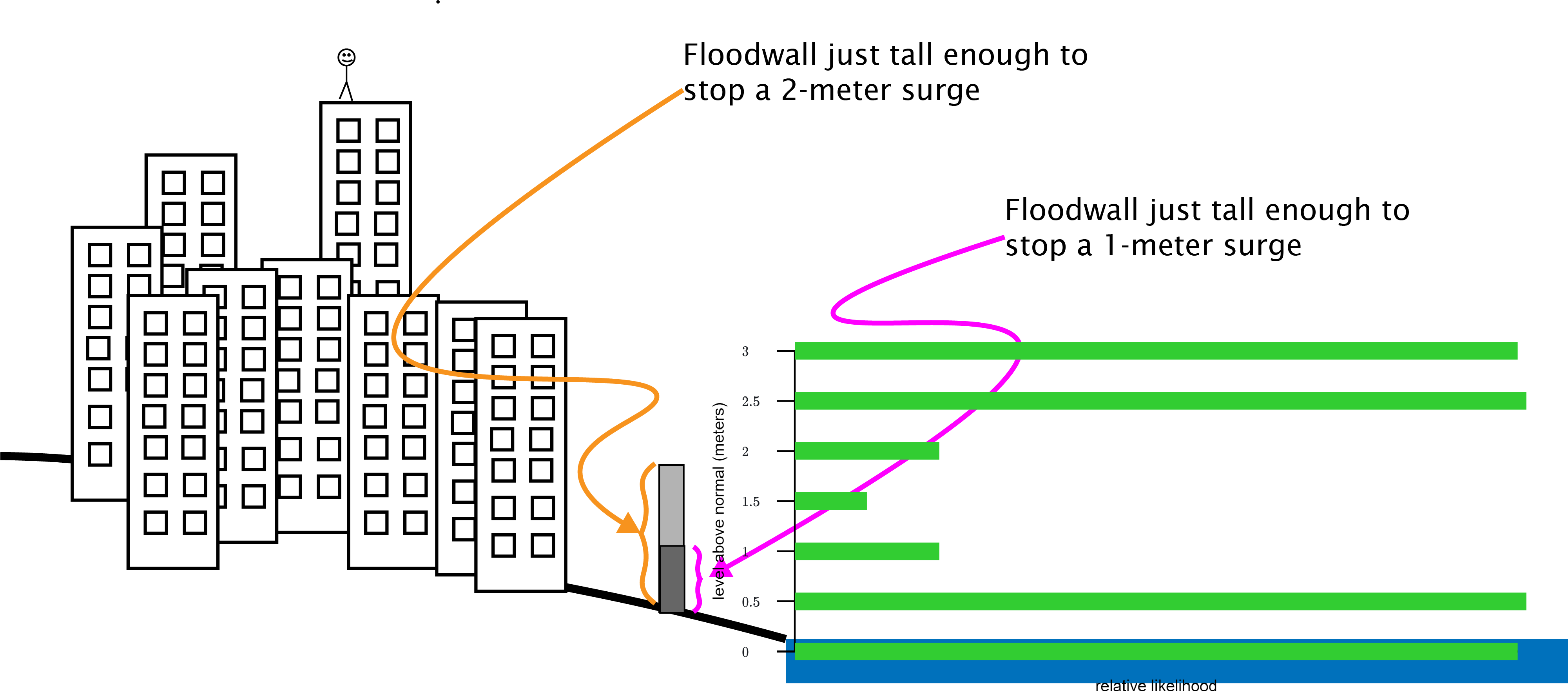
The mayor’s idea is to build a seawall between the city and the river. The wall will be impervious to water and will stand some meters higher than the river’s normal level. Its foundations will be anchored in the bedrock that lies several feet below the city’s sandy soil. So when the river rises, the water will be held behind the wall, keeping the city’s people and buildings dry. When finished, it will look something like this:

To build her seawall, the mayor must first resolve a very basic issue: Just how tall should the seawall be? As an elected politician, dependant for her job on campaign contributions from wealthy city residents and on votes from everyone else, this question is critical. The cost to taxpayers of the seawall will be exorbitant, and these costs will rise with the height of the wall. The mayor, then, will want to build the wall just high enough to keep the city dry most of the time, and no higher. So how high is that? This is a difficult question to answer, because no one can know how strong the hurricanes that pass near the city will be in any given year. A seawall too tall, on the one hand, will be more than is needed against the relatively small storms of most years. A seawall too short, on the other hand, will fail in the face of a large storm.
To depict the mayor’s choice and its stakes, we’ll use a probabilistic model of uncertainty. Suppose that the city’s historical records show that in most years, no storm pushes the river’s waters above their normal level. Storms that push the river about one-half a meter above its normal level, on the other hand, occur occasionally. Storms flooding the river to a level about one meter occur somewhat less frequently than that. Storms pushing the river to one-and-one-half meters above normal occur less frequently than that, and so on up to the rarest event, which has occurred only once in recorded history and in which the rivers surges to three meters above its normal level. Thus, supposing that surges in the river’s level continue to occur at roughly the frequency of those surges seen in the past, the relative likelihood in any given year with which the river will rise to each possible height above its normal level looks something like this:
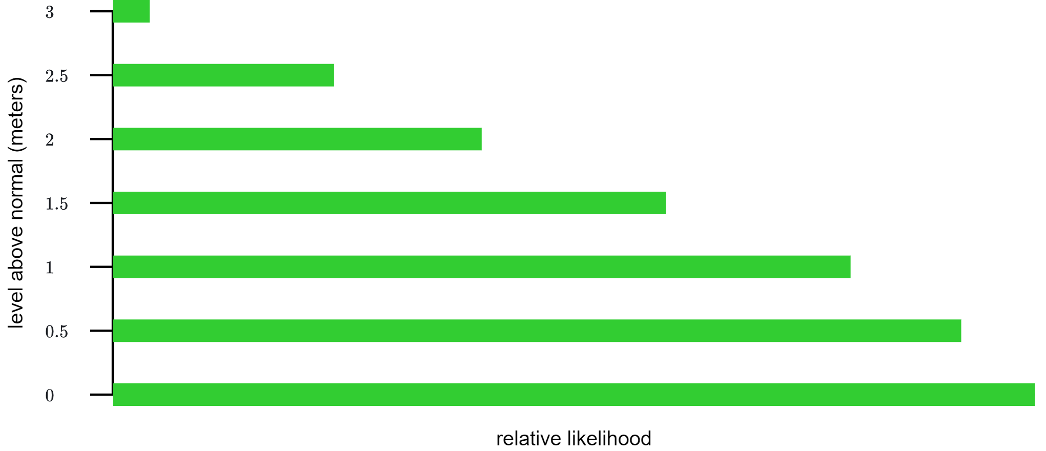
The key idea this graph depicts – and the key idea that probabilistic models of uncertainty depict in general – is that it is possible to be uncertain about which of a set of events will occur, yet to have definite beliefs about the relative likelihoods of each of those events. Our imaginary mayor, for instance, does not know how high the river will rise in any given year after she constructs her seawall. But she has definite beliefs about how likely a surge in the river’s level of any given height is to occur relative to a surge of any other height. Examining the figure above, for instance, you can see that she believes that the river surging to one meter above its usual level is about twice as likely as the river surging two meters above its usual level.
Superimposing our graph of the relative likelihoods of river levels of different heights on our cartoon sketch of the mayor and her city helps to clarify the implications for decision making of the information about relatively likelihoods that a probabilistic model depicts. Recalling that our mayor needs to decide how high to build her seawall, consider the choice between a seawall just tall enough to protect the city from a one-meter surge in the river versus a seawall just tall enough to protect the city from a two-meter surge, like this:
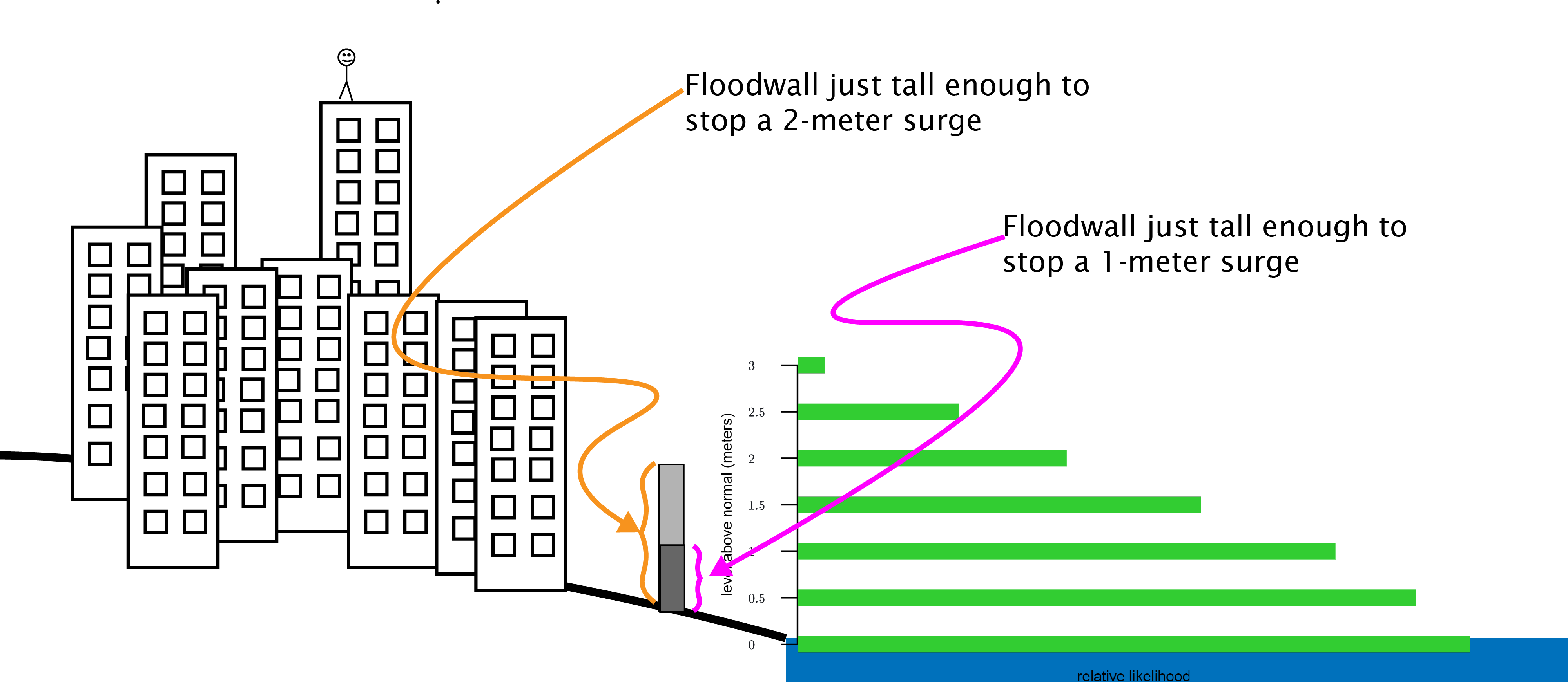
Notice that a difference in performance between these two seawalls only occurs in very particular circumstances – i.e. when a storm raises the level of the river either 1.5 or 2 meters above its typical level. In contrast, surges smaller than one meter and surges larger than two meters result in the same outcome regardless of which of these two possible walls are built. So, in choosing between a one-meter a two-meter wall, what really matters to the mayor is how likely a surge of 1.5 or 2 meters is. If surges in that narrow range are relatively likely, the additional cost of the taller seawall may be well worth it.
For instance, suppose that, in contrast to what we assumed above, only very big (higher than 2.5 meters) and very small (0.5 meters or less) surges in the river’s level are likely, while middle-range surges (between 1 and 2 meters) are very unlikely. Something like this:
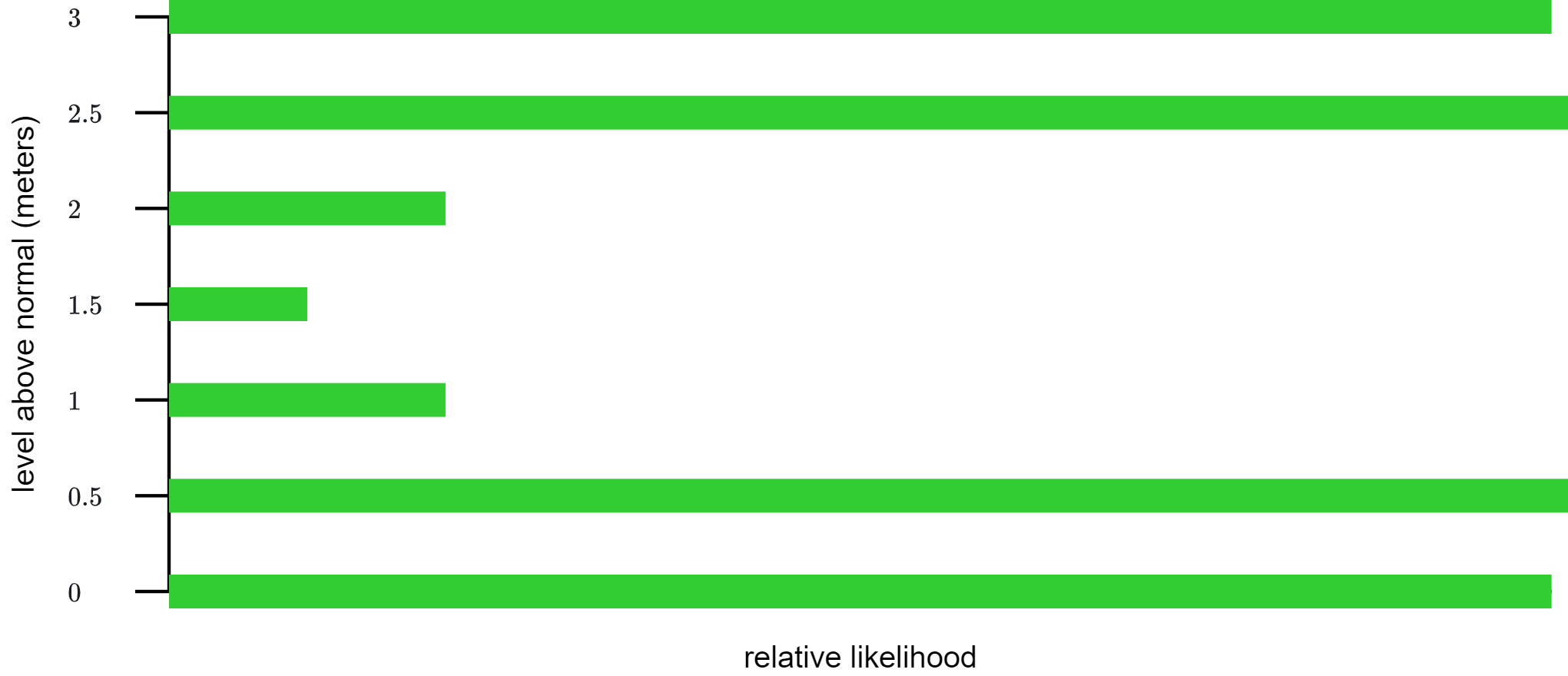
Superimposing this graph on our sketch of the mayor and her city shows that the choice between a 1-meter seawall and 2-meter seawall looks quite different:
In this case, the mayor gains relatively little by increasing her seawall from just high enough to stop a 1-meter surge to just high enough to stop a 2-meter surge.
Defining Probabilistic Models of Uncertainty
A probabilistic model of uncertainty has two elements: A description of a set of exhaustive and mutually exclusive possible events, and a probability distribution that depicts the relative likelihood with which each possible event will occur.
For example, we can model the mayor’s uncertainty about the height to which the river will surge above its normal level in any given year using the following probabilistic model of uncertainty:
There are two things to notice about this model. First, the list of possible events is highly simplistic, in that there are only seven possible heights above its usual level to which the river will surge. These heights, moreover, are laid out in precise, half-meter intervals. While a more realistic model is possible, the simplistic model here is useful for illustrating the most important feature of any probabilistic model’s description of possible events: Any such description must be exhaustive (i.e. it must specify all possibilities), and it must be precise about which events are mutually exclusive of each other. By making the simplistic assumption that the river will rise to exactly one of only six particular heights, and by specifying each of these six particular heights, this model of flooding meets both of these requirements.1
Second, the probability distribution this model uses to depict the events’ relative likelihoods amounts to a list of numbers, with one number assigned to each possible event. More generally:
More Examples of Probabilistic Models
This section illustrates key aspects of probabilistic models used in PPT through a series of examples. We’ll start with what might be the simplest probabilistic model possible – a model of the uncertainty you face when you flip a coin. When you flip a coin, the outcome – i.e. whether the coin lands heads-up or tails-up – is uncertain. Moreover, each of these two outcomes is just as likely to occur as the other. Here is a model that captures both of these aspects of the uncertainty about the outcome of a coin flip.
Why does this model assign the number 0.5 as the probability for both “heads-up” and “tails-up”? Recall the two rules of probabilities: Each probability must be a number between 0 and 1, and the sum of all the probabilities assigned to the full list of mutually exclusive events must be 1. Since we want to depict each face of the coin as equally likely to occur, the numbers assigned as probabilities to those events must be equal to one another. And there is only one number between 0 and 1 that when added to itself is 1 – i.e. 0.5.
A similar line of thinking is at work in the only slightly more complex uncertainty faced when one rolls a six-sided die. The die has six faces, and thus there are six outcomes instead of the two outcomes that can occur when one flips a coin. Each face is equally likely to occur. Thus, since each probability must be a number between 0 and 1 and since the six probabilities must sum to 1, the probability assigned to each face of the die must be \frac{1}{6}.
Possible Events
The die will land with one of its six faces up.
Probability Distribution
| Event | Probability |
|---|---|
|
\frac{1}{6} \frac{1}{6} \frac{1}{6} \frac{1}{6} \frac{1}{6} \frac{1}{6} |
Pause and complete check of understanding 1 now!
The two examples above are simple and clear but do not obviously resemble any important aspects of politics. Can the uncertainties we face in politics – which are vastly more complex and ambiguous than the uncertainty involved in flipping a coin or rolling a die – be depicted using a probabilistic model?
At the time of this writing (October of 2024), there is apprehension across the world that the Peoples Republic of China might launch a military invasion of the island of Taiwan at some point in the next several years. No one, excepting perhaps the paramount leaders of the Chinese Communist Party, can know for sure whether such an invasion will occur, or whether an invasion, if attempted, will end in a successful military occupation of Taiwan by the PRC.
The complexity of a potential military invasion of Taiwan by the PRC and the possible reactions to an invasion by the world’s other militaries is overwhelming. Hundreds of thousands of soldiers, pilots, and sailors from dozens of nations would likely be involved in fighting triggered by an invasion, and the fighting would set off cascades of reactions in multiple non-military domains – including in trade flows and trade routes, diplomatic relations and alliances between nations, and the balance of political power between competing factions within multiple nations. Such an invasion could even trigger an exchange of nuclear weapons, opening up the possibility for levels of destruction that could lead to the collapse of nation-states.
Can such a bewildering tangle of momentous possibilities be reasonably depicted using a probabilistic model? Yes, partially. Consider two simple questions about a possible invasion:
- Will the PRC launch an invasion of Taiwan at some point between now and October 1 of 2028?
- If the PRC launches an invasion of Taiwan at some point between now and October 1 of 2028, will that invasion culminate in a successful military occupation of Taiwan by the PRC at some point between now and October 1 of 2030?
These two questions set aside all of the uncertainties of a potential invasion except for two definite and conceptually simple questions – within a certain period of time, will there be an invasion, and if so will that invasion succeed? These questions are deliberately phrased so that they each have exactly two possible answers – i.e. “yes” or “no”. Thus we can use a probabilistic model just as we use all other PPT modeling tools: To depict one aspect of an otherwise un-manageably complex reality.
Pause and complete check of understanding 2 now!
One thing about the model above is absolutely essential to recognize: In the absence of a large number of previous cases of potential invasions like the PRC’s potential invasion of Taiwan, we have no evidentiary basis for deciding whether any precise numerical probabilities assigned by the model are reasonable or valid. Consider, in contrast, the heights to which a river might flood in any given year. Using a historical record of the river’s flood levels over several decades, we can calculate the frequency with which each flood level has occurred and estimate probabilities for each possible flood level in a future year accordingly. No such calculation is possible for an event as historically idiosyncratic as a potential invasion of Taiwan by the PRC.
Thus it does not make sense to interpret the probabilities in the above model as representations of objectively knowable relative likelihoods. Instead, models of uncertainties like the one we currently face about the future of Taiwan – i.e. uncertainties in which we have little or no empirical basis from which to determine relative likelihoods – are best interpreted as depictions of subjective beliefs that different persons might hold about uncertain events. For instance, military and political leaders throughout the world differ widely in their assessments of how likely the PRC is to launch an invasion of Taiwan sometime in the next several years and the PRC’s prospects of success if it invades. So, although a model like the one above is not useful for depicting the actual likelihood of a PRC invasion of Taiwan, it can be useful for depicting variations across political leaders in these assessments. Specifically, it could be used to depict some leaders who believe an invasion is very likely to occur but very unlikely to succeed if it does occur, and thus have beliefs like this…
| Event | Probability |
|---|---|
| no invasion by 2028 | 0.25 |
| invasion by 2028 but no successful occupation by 2030 | 0.675 |
| invasion by 2028 and successful occupation by 2030 | 0.075 |
…and other leaders who believe an invasion is very unlikely to occur but very likely to succeed it does occur, and thus have beliefs like this:
| Event | Probability |
|---|---|
| no invasion by 2028 | 0.75 |
| invasion by 2028 but no successful occupation by 2030 | 0.025 |
| invasion by 2028 and successful occupation by 2030 | 0.225 |
More generally, differences between persons in their beliefs, hunches and suppositions in response to uncertainty are a ubiquitous source of conflict in politics. Consider, for instance, Americans’ beliefs about the rightful and legitimate winner of the 2020 presidential election. Most (perhaps all?) Americans do not have the ability to directly check the validity of the numerous processes of voting and ballot counting that culminated in the 2020 election outcome. Instead, their beliefs about the legitimacy of the 2020 election depend on what they have heard about the election from voices in the media, and which of those voices they trust. Since November of 2020, a small but powerful faction of Republican politicians and right-wing media outlets have insisted that the election was fraudulent and Donald Trump was the rightful winner. A somewhat larger group of moderate Republicans, Democrats and mainstream and left-wing media outlets have maintained that the election was valid and Joe Biden was the rightful winner. The result is a variety of beliefs in the general population about who was the actual and rightful election winner.
An organization called Bright Line Watch, for instance, has run a twice-yearly poll of Americans since 2017 meant to monitor the state of American democracy. In an October 2022 poll, they asked a sample of about 2700 respondents “Do you consider Joe Biden to be the rightful winner of the 2020 presidential election or not the rightful winner?” Respondents were given the option to select one of “Definitely the rightful winner”, “Probably the rightful winner”, “Probably not the rightful winner”, or “Definitely not the rightful winner”. Weighting the sample to adjust for under-response to surveys by some groups, the results suggest the following:2
| Belief about the 2020 election | Percentage of Americans holding that belief |
|---|---|
| Biden was definitely the rightful winner | 47.0\% |
| Biden was probably the rightful winner | 19.2\% |
| Biden was probably not the rightful winner | 15.4\% |
| Biden was definitely not the rightful winner | 18.4\% |
We can depict any one of these four different beliefs about the rightful winner of the 2020 presidential election using a probabilistic model as follows:
Pause and complete check of understanding 3 now!
Modeling Multiple Uncertainties
Thus far, you’ve only seen probabilistic models of single uncertainties. For instance:
- How high will the river rise in the next hurricane?
- When flipping a coin, which face will land heads-up?
- In an election in which two or more candidates are running, which candidate will win?
- Will the PRC launch an invasion of Taiwan at some point between now and 2028?
In practice, however, we often want to model political situations in which actors face multiple uncertainties.
Consider, for instance, the uncertainties politicians face when they decide whether to initiate the construction of large infrastructure projects, such as flood-control systems, rail transit networks, deep sea ports and power generation facilities. Big infrastructure projects have long timelines. In 1965, for instance, when the U.S. Congress authorized construction of the levees and floodwalls in New Orleans that hurricane Katrina would overwhelm 40 years later, the engineers designing the project estimated that construction would take at least 10 years. And as it turned out, construction was not complete until the 1990s. These very long timelines create multiple, related uncertainties for the politicians who choose whether, how and when to initiate big infrastructure projects. For instance, if a big, multi-year project is to be completed, the government must spend money on the project one year after the next, for several successive years. And whether and how much the government spends on anything in any given year depends on which political factions control the government in that year and which expenditures those factions find politically advantageous. So, whether a big project that a politician starts today ultimately pays off in a functioning and complete piece of infrastructure several years down the line hinges on the uncertain course during many successive years of both political power and the incentives of whoever holds political power.
To show how to model multiple uncertainties, we’ll imagine a politician who starts an infrastructure project today, but is uncertain who will have power tomorrow, and whether whoever has power tomorrow will continue to fund the project started today. Imagine specifically that the politician believes that one of three political factions – labeled A, B, and C – will hold the power to direct the government’s spending tomorrow. Further, suppose that whichever faction has power tomorrow will take one of two alternative actions: fund the infrastructure project the politician has started today or do not fund the project.
The first thing you need to know is that the definition of a probabilistic model that you learned earlier in this lesson applies to multiple uncertainties just as it does to single uncertainties. Specifically, a probabilistic model of multiple uncertainties consists of a list of all mutually exclusive possible resolutions of the uncertainties and a probability distribution over those resolutions. For instance, in our simplistic depiction of a politician’s uncertainty about which faction will hold power tomorrow and whether the faction that holds power will fund or not fund an infrastructure project, there are six mutually exclusive possible resolutions of the politician’s uncertainty…
- Faction A holds power and funds the project.
- Faction A holds power and does not fund the project.
- Faction B holds power and funds the project.
- Faction B holds power and does not fund the project.
- Faction C holds power and funds the project.
- Faction C holds power and does not fund the project.
…and so we can specify a probabilistic model of this uncertainty by assigning a probability to each of these resolutions, making sure that the probabilities we assign sum to 1. For instance:
| Event | Probability |
|---|---|
| Faction A holds power and funds the project. | \frac{1}{6} |
| Faction A holds power and does not fund the project. | \frac{1}{6} |
| Faction B holds power and funds the project. | \frac{1}{6} |
| Faction B holds power and does not fund the project. | \frac{1}{6} |
| Faction C holds power and funds the project. | \frac{1}{6} |
| Faction C holds power and does not fund the project. | \frac{1}{6} |
This brute-force approach – i.e. listing all possible resolutions and assigning a probability to each resolution directly – is completely valid. But as a technique for building a model of multiple uncertainties, it’s rarely useful. When we model a collection of multiple uncertainties, we typically want to depict interdependence between the individual uncertainties making up that collection. More precisely, we want to depict the idea that the way that some of the uncertainties are resolved affects the relative likelihoods of the different possible resolutions of the other uncertainties. For example, imagine that political factions A, B and C differ in the extent to which they rely on political support from trade unions representing construction workers, with faction A wholly reliant on construction-trade unions, B somewhat reliant, and C not at all reliant. Since big infrastructure projects create lots of jobs for construction workers, we might then suppose that the project is most likely to be funded if A takes power, less likely to be funded if B takes power, and least likely to be funded if C takes power. It’s difficult to model that kind of interdependence between uncertainties using the brute-force approach demonstrated above. So, in this section you’ll learn a set of concepts and techniques that make modeling interdependencies between multiple uncertainties easier.
The major concepts you’ll learn are:
Joint Uncertainty, Joint Events, Joint Probability
The foundational move for everything you’ll learn in this section is to think about multiple uncertainties as joint uncertainty. Joint uncertainty is uncertainty about how all of a collection of single, distinct uncertainties will be resolved. For example, the politician’s uncertainty about which faction will hold power tomorrow and whether the faction in power tomorrow will fund the project she starts today can be thought of as uncertainty about how both of two distinct uncertainties will be resolved:
- Which faction will hold power tomorrow?
- Will the faction that holds power tomorrow fund the project?
In a case like this, in which multiple uncertainties can be thought of as joint uncertainty over two distinct uncertainties (which is the only case we’ll work with in detail in this course), joint uncertainty can be visualized using a grid. For instance:
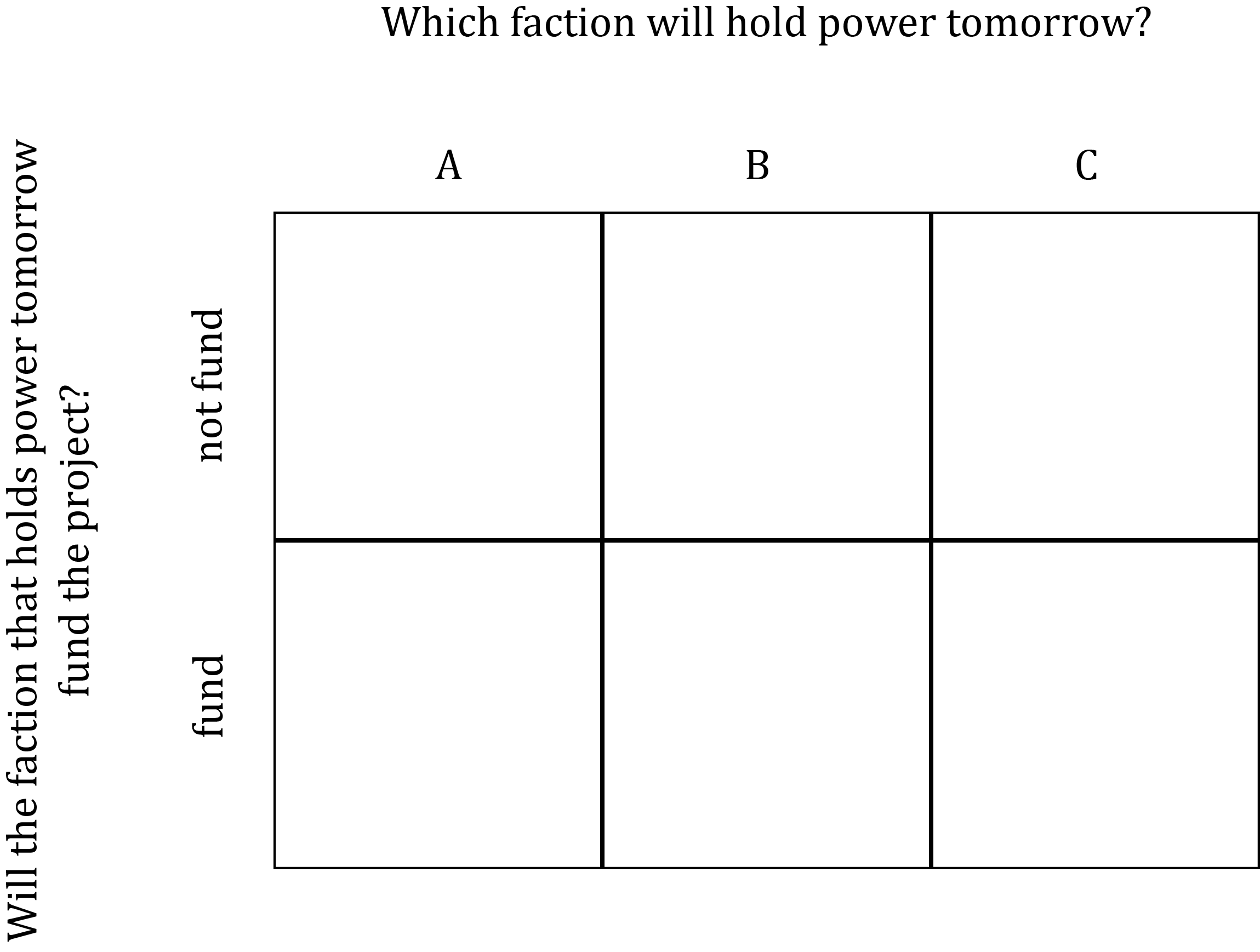
The key thing that a grid representation of joint uncertainty does is depict each of two distinct uncertainties as occupying space along a separate axis. For instance, the grid above depicts uncertainty about which faction will hold power along the horizontal axis and uncertainty about whether whichever faction holds power will fund the project along the vertical axis.
When we depict joint uncertainty using a grid, the set of mutually exclusive possible resolutions of the uncertainty are represented by the cells in the grid. These possible resolutions of the uncertainty are called joint events. More generally, a joint event is an event composed of one possible realization from each of a collection of distinct uncertainties. For instance, the top-left cell highlighted in yellow here…

…represents the joint event in which the uncertainty about who will hold power tomorrow is resolved as “A”, and the uncertainty about whether the faction that holds power tomorrow will fund the project is resolved as “not fund”.
The joint events represented in the cells of the grid amount to an exhaustive list of the mutually exclusive possible resolutions of the joint uncertainty. Thus by assigning a probability to each cell of the grid, with the probabilities in the cells together summing to 1, we create a probability distribution that models the joint uncertainty depicted in the grid. For instance:
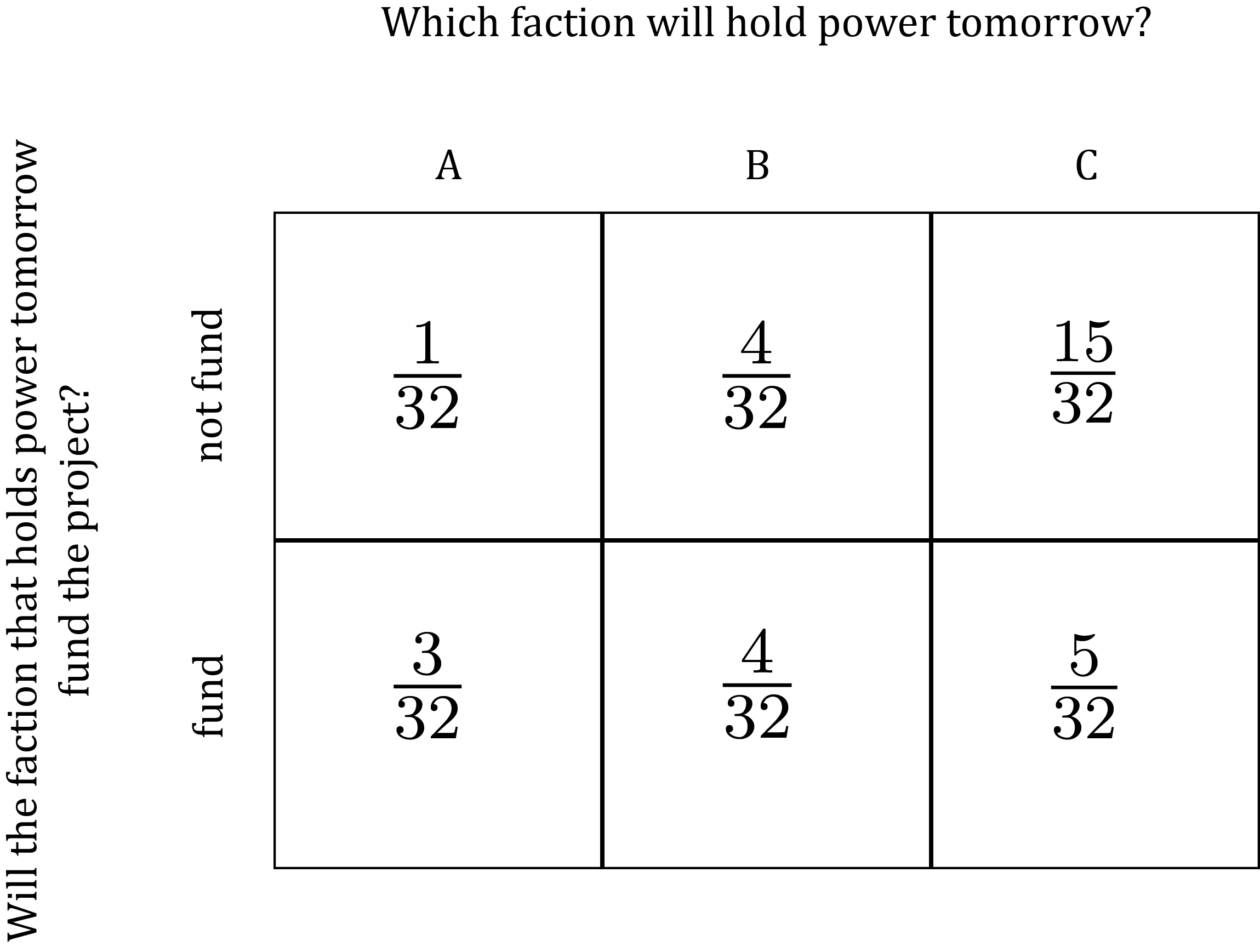
The probability assigned to a joint event is called a joint probability. In general, when (for instance) X, Y, and Z are possible realizations of three distinct uncertainties, we use P(X \& Y \& Z) to denote the joint probability that X and Y and Z occur. So, for example, if we want to show our model of the politician’s uncertainty without specifying definite numerical values for the probabilities, we can write something like this:

Here’s a summary of these concepts:
Pause and complete check of understanding 4 now!
Marginal Uncertainty and Marginal Probability
Modeling multiple uncertainties as joint uncertainty allows us to analyze each of a collection of distinct uncertainties in isolation from the others. For example, consider our model of the politician’s uncertainty about which faction will hold power tomorrow and whether the faction that holds power will fund the infrastructure project:
Imagine that a young staffer who works for the politician has come to her for advice.
I’m trying to figure out,
the staffer says,
who I should be making connections with to secure my future career. Given that we don’t know who will be in power tomorrow and whether they will fund your signature infrastructure project, I’m really not sure.
Suppose the politician responds by saying:
If you’re thinking about your future career, forget about the infrastructure project! All you need to worry about is which faction will hold power tomorrow. No matter what they do with the project, the faction in power is the faction you want to be working for.
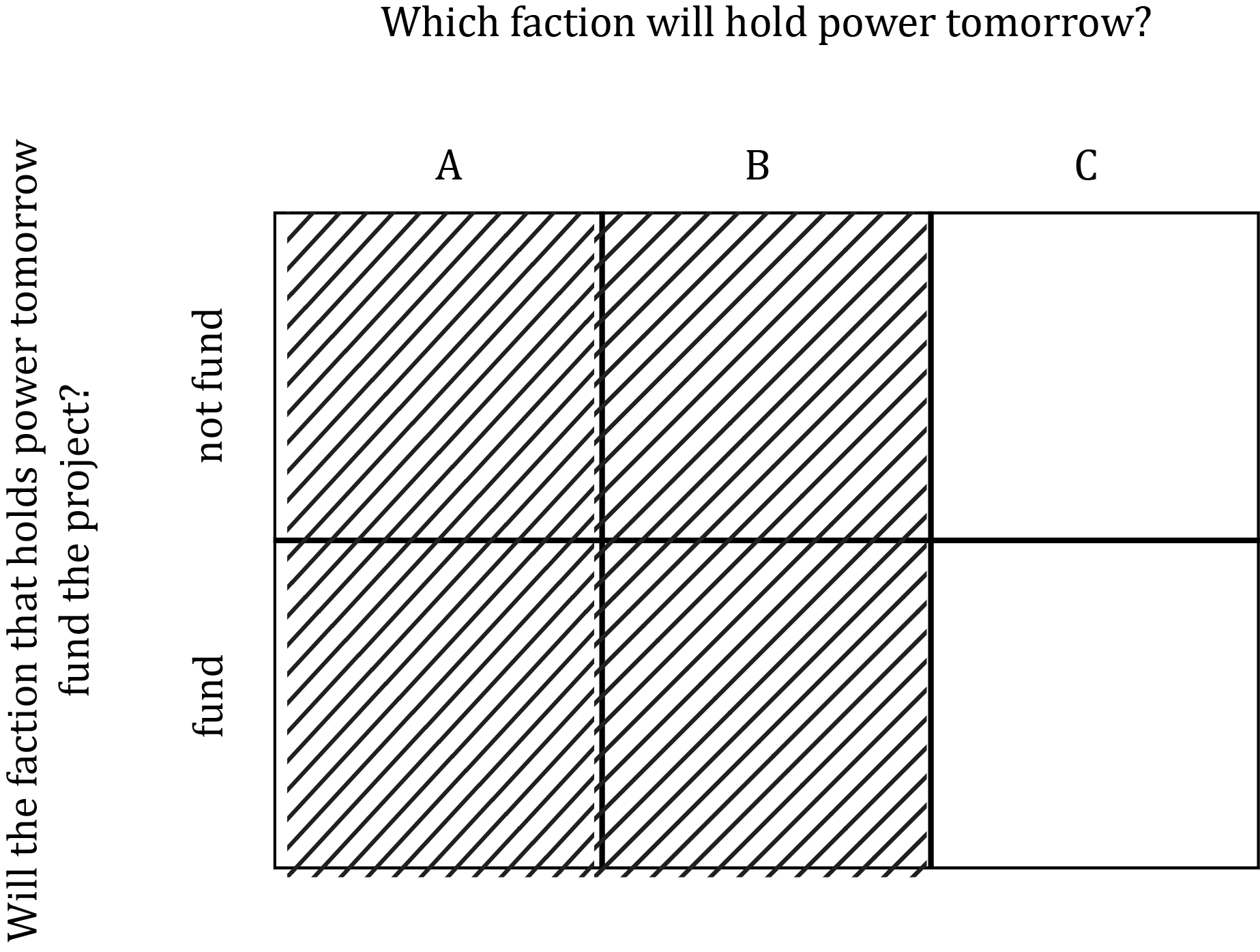
In effect, the politician is telling his staffer to focus only on the uncertainty about which faction will hold power next year. We can use our grid depicting joint uncertainty to depict the single uncertainty that the politician is telling her staffer to focus on like this:
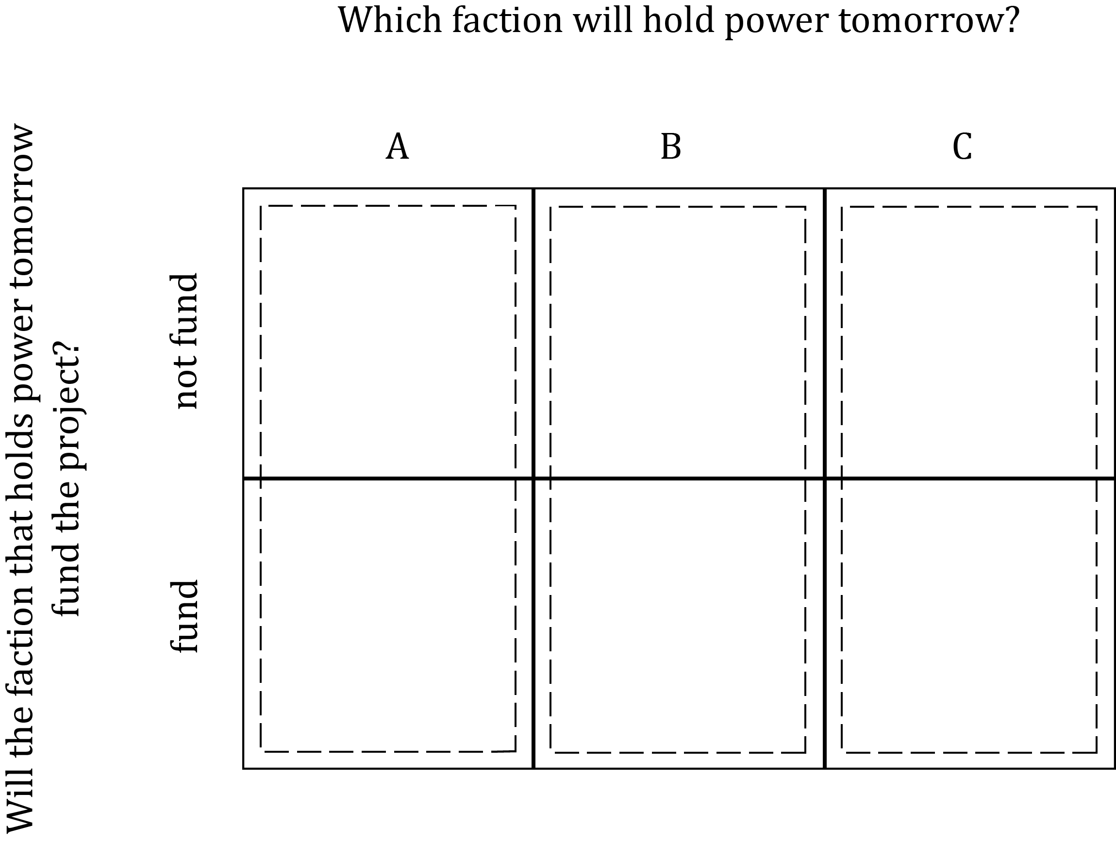
In this diagram, uncertainty only about which faction will hold power tomorrow is equivalent to uncertainty about which of the three dashed rectangles will contain the cell representing the resolution of the joint uncertainty. For instance, the uncertainty only about which faction will hold power tomorrow is resolved as “A” if the joint uncertainty is resolved either as the top-left event “not fund & A” or as the bottom-left event “fund & A”.
We call uncertainty like this – i.e. uncertainty about just one of a collection of distinct uncertainties – marginal uncertainty. A probabilistic model of marginal uncertainty is just like any other probabilistic model. Specifically, it consists of an exhaustive list of mutually exclusive possible resolutions of the marginal uncertainty, with probabilities assigned to these possible resolutions that together sum to 1. The probabilities assigned in a model of marginal uncertainty are called marginal probabilities. We use the notation P(X) to refer to the marginal probability that a marginal uncertainty is resolved as the event X.
For instance, we can use our grid to model the staffer’s marginal uncertainty just about which faction will hold power tomorrow like this:
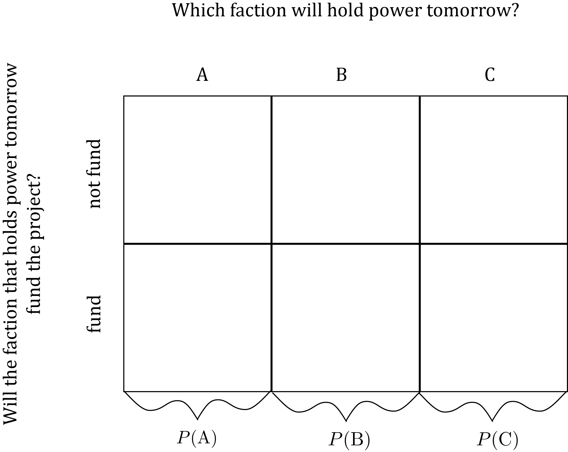
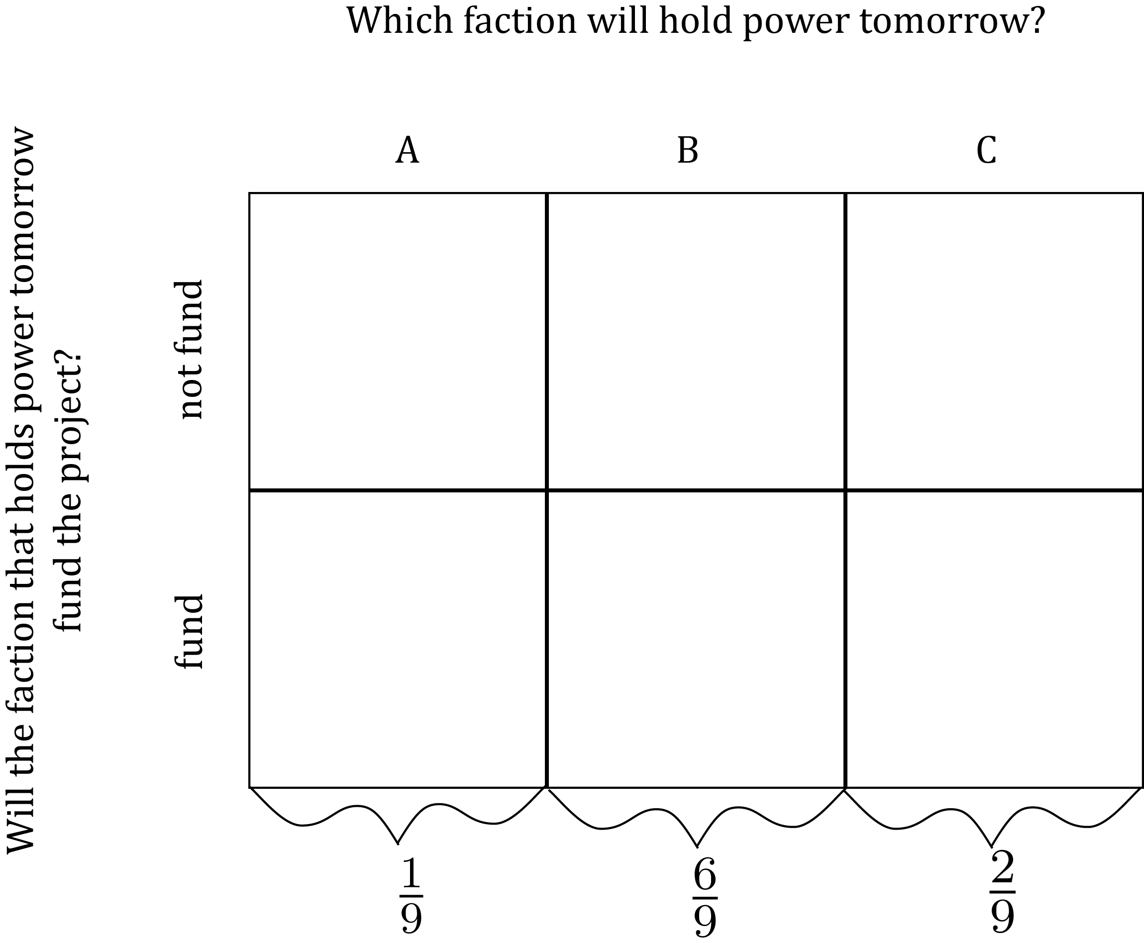
The diagram depicts the three mutually exclusive possible resolutions – A, B, and C – of the marginal uncertainty about who will hold power tomorrow, with probabilities P(A), P(B) and P(C). Since A, B and C together make up the exhaustive list of mutually exclusive resolutions of the uncertainty about who will hold power tomorrow, their probabilities must sum to 1, i.e.: P(A) + P(B) + P(C) = 1 For instance:
Similarly, we can model the marginal uncertainty just about whether the project will be funded like this:
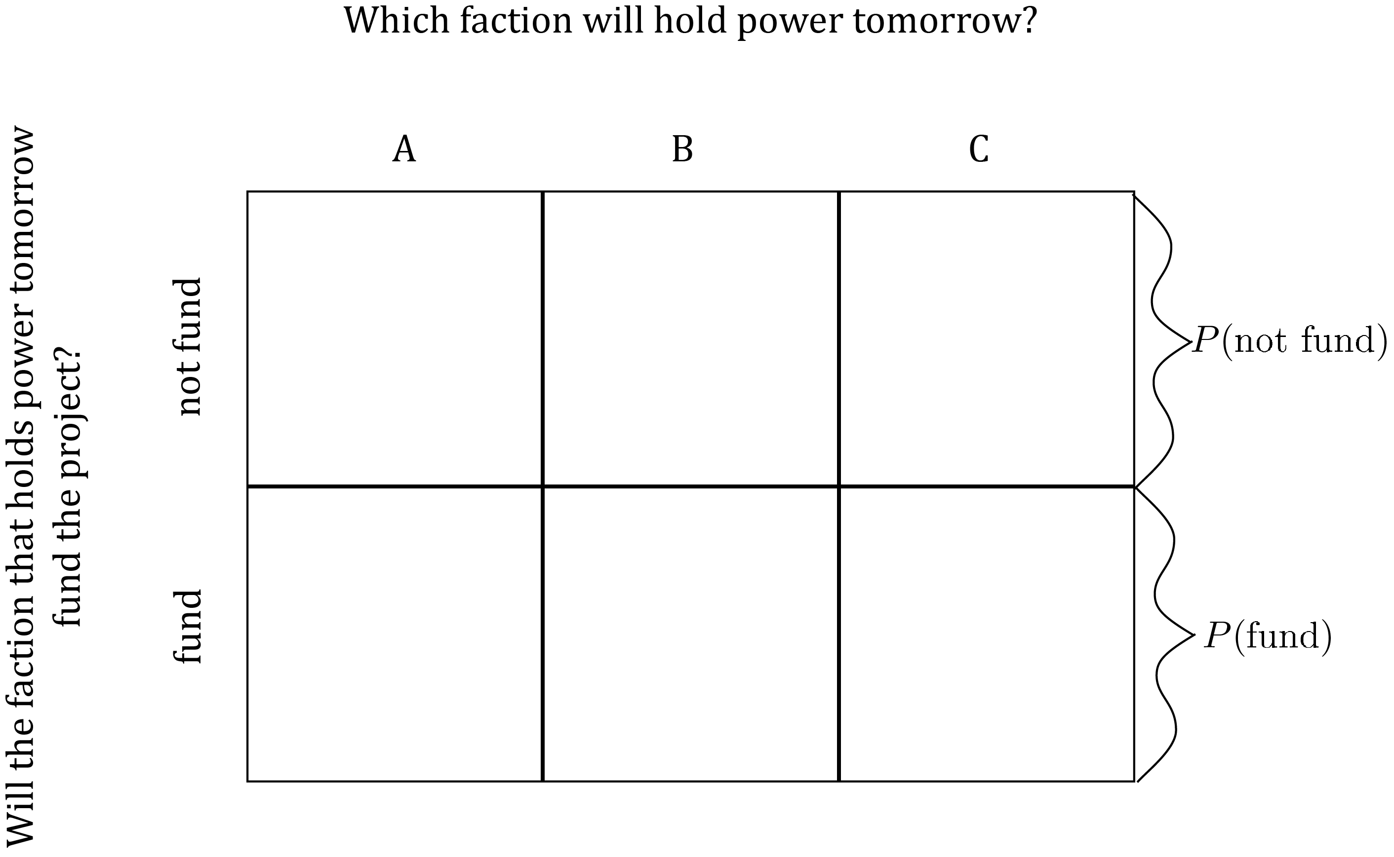
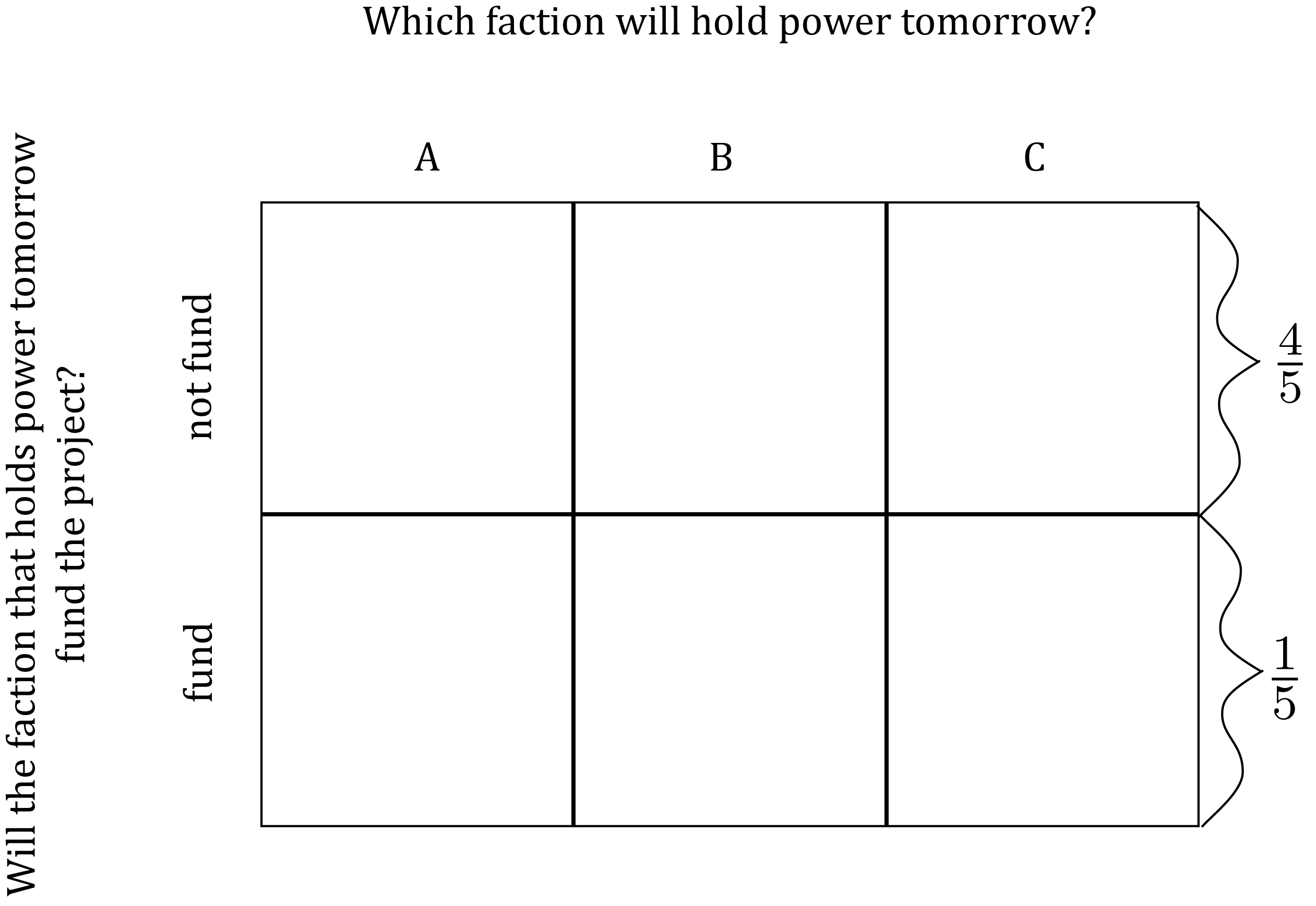
Since “fund” and “not fund” together make up the exhaustive list of mutually exclusive resolutions of the marginal uncertainty about whether the project will be funded, it must be that P(\text{not fund}) + P(\text{fund}) = 1 For instance:
There is a connection between marginal probabilities and joint probabilities that it’s essential to know about. To understand it, consider the marginal uncertainty just about whether the project will be funded. Notice that the resolution “fund” of that marginal uncertainty is equivalent to the event that the joint uncertainty about which faction will hold power and whether the project will be funded is resolved as one of “fund & A” or “fund & B” or “fund & C”. And since those three events are mutually exclusive, the probability that one of them occurs is equal to the sum of their probabilities. Thus we have the identity: P(\text{fund}) = P(\text{fund \& A}) + P(\text{fund \& B}) + P(\text{fund \& C}) More generally, take any joint uncertainty over how both of two distinct uncertainties will be resolved. Let X be one possible resolution of one of the two distinct uncertainties, and let Y_1, Y_2, \ldots, Y_N be the exhaustive list of the mutually-exclusive possible resolutions of the other distinct uncertainty. Then P(X) = P(\text{$X$ \& $Y_1$}) + P(\text{$X$ \& $Y_2$}) + \cdots + P(\text{$X$ \& $Y_N$}) In words, the marginal probability that the marginal uncertainty about one issue is resolved as X is equal to the sum of the joint probabilities of all the mutually exclusive joint events in which X occurs.
This identity means that the marginal probabilities in a model of joint uncertainty constrain, but do not fully determine the joint probabilities. For instance, suppose we model (a) the marginal uncertainty just about which faction will hold power and (b) the marginal uncertainty just about whether the project will be funded like this:
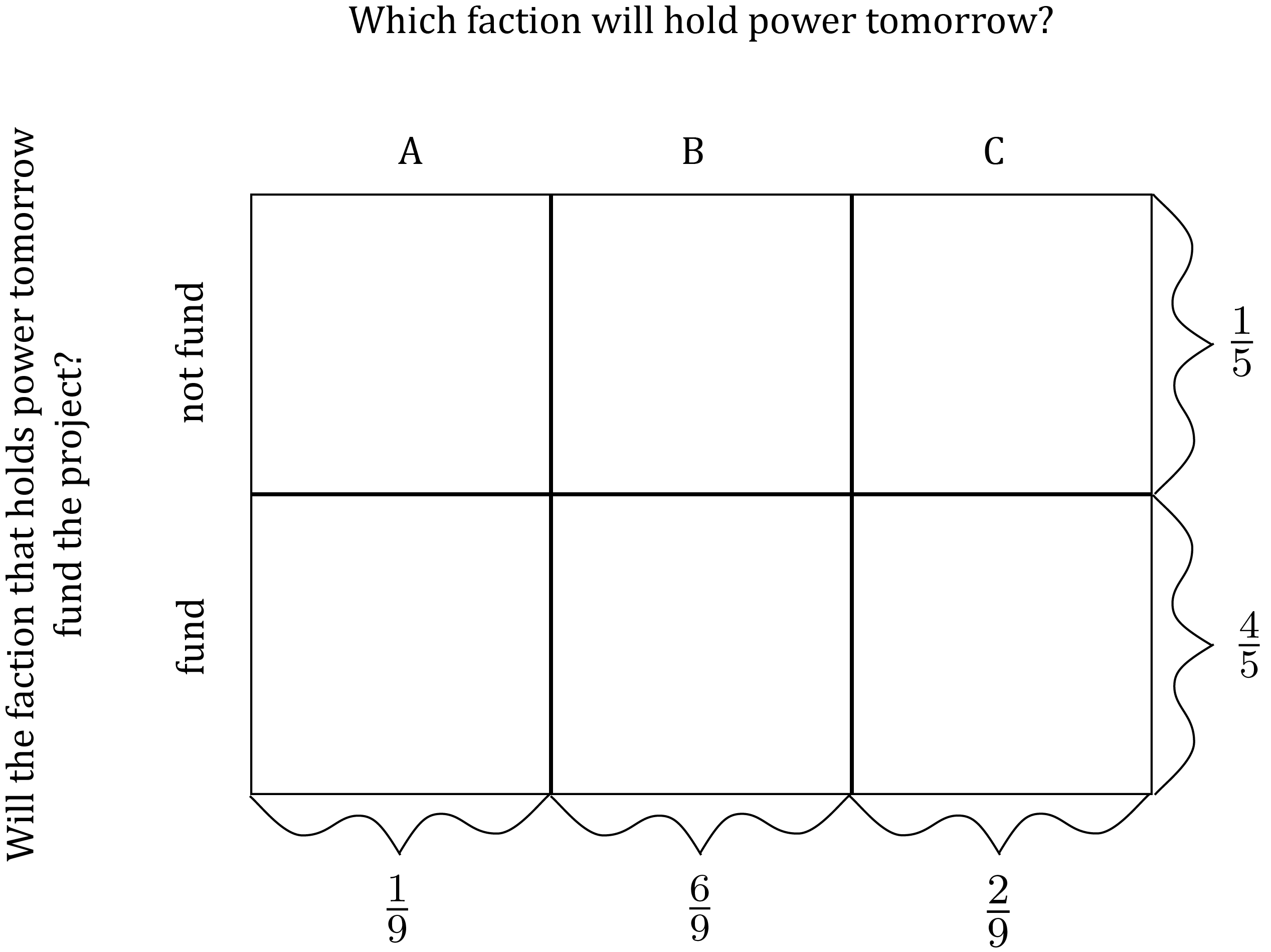
Then the identity above requires that the joint probabilities must satisfy all the following equalities: \begin{gather*} P(\text{not fund \& $A$}) + P(\text{not fund \& $B$}) + P(\text{not fund \& $C$}) = \frac{1}{5} \\\\ P(\text{fund \& $A$}) + P(\text{fund \& $B$}) + P(\text{fund \& $C$}) = \frac{4}{5} \\\\ P(\text{not fund \& $A$}) + P(\text{fund \& $A$}) = \frac{1}{9} \\\\ P(\text{not fund \& $B$}) + P(\text{fund \& $B$}) = \frac{6}{9} \\\\ P(\text{not fund \& $C$}) + P(\text{fund \& $C$}) = \frac{2}{9} \\\\ \end{gather*}
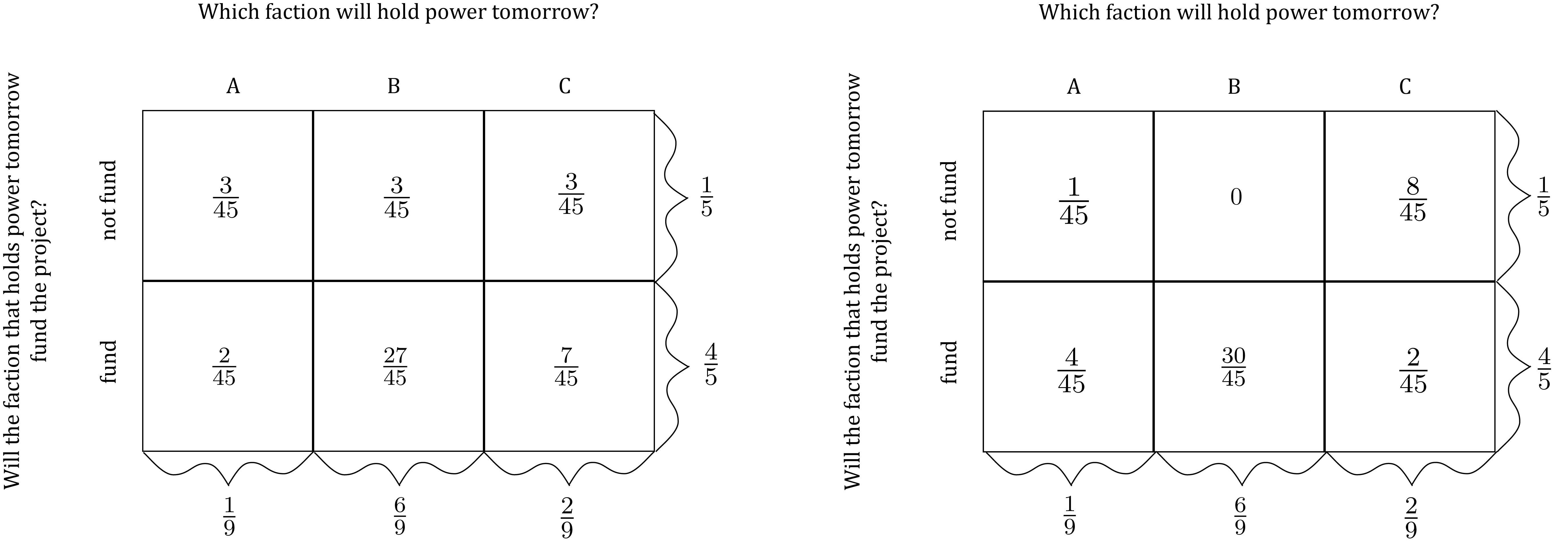
There are multiple arrays of values of the joint probabilities that can satisfy all of the above equalities. For instance, here are two different sets of values for the joint probabilities that are both consistent with the marginal probabilities assigned above (i.e. they sum across the rows and columns correctly):
Here is a summary of the major concepts in this section:
Pause and complete check of understanding 5 now!
Conditional Uncertainty and Conditional Probability
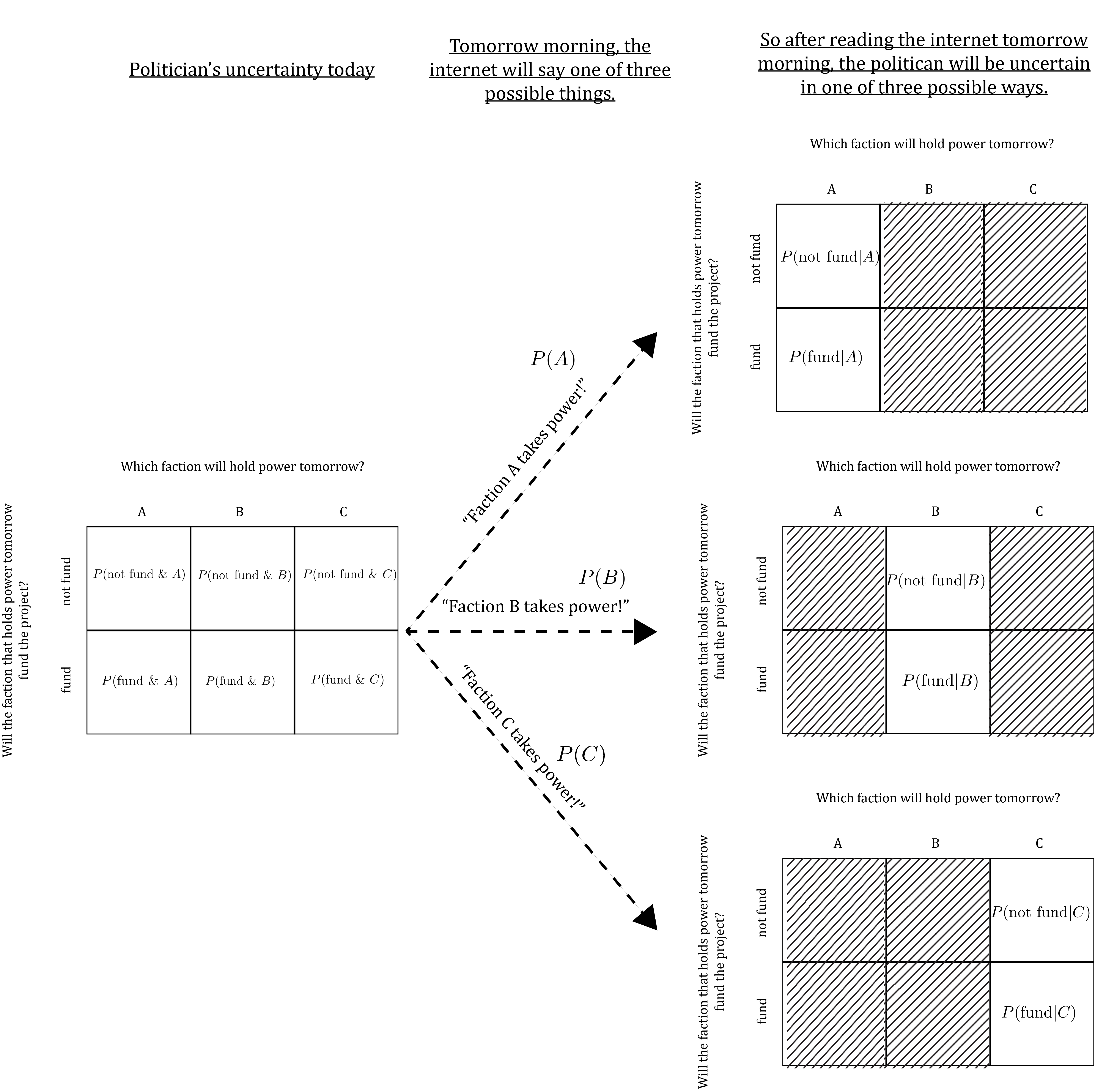
Continue to imagine our politician who is uncertain about which faction will hold power tomorrow and whether the faction that holds power will fund the infrastructure project the politician starts today. Imagine this politician getting ready to go to bed at the end of what we’re calling “today”. Suppose that just before she lays down to sleep, she pauses to think about what will happen when she wakes up tomorrow. She knows that while she sleeps, the final ballots will be counted in an election that will determine which faction holds power tomorrow. And she knows that when she wakes up tomorrow, and after she has enjoyed a cup of coffee, she will go to her favorite news site on the web and will immediately learn which of the three factions has won the election and taken power. More specifically, she knows she will see one of three headlines:
- “Faction A takes power!”
- “Faction B takes power!”
- “Faction C takes power!”
At that point, whichever faction has won the election will not have had time to pass any legislation. So, as the politician is getting ready to go to bed today and thinking about what she will know tomorrow just after she drinks her coffee and looks at the internet, she knows that her uncertainty will be partially resolved. It looks like this:

Each of the three partially-obscured grids on the right-hand side of this diagram depict conditional uncertainty. Conditional uncertainty is uncertainty about one or more issues, conditional on knowledge of how some other issues were, are, or will be resolved. For instance, examine the grid in the bottom right of the diagram above, which depicts the politician’s uncertainty about whether the project will be funded, conditional on the knowledge that faction C is in power tomorrow:
Conditional on the knowledge that faction C is in power, four of the six outcomes in the grid depicting the politician’s joint uncertainty are ruled out. Hence, the grid depicting this conditional uncertainty has four cells crossed out. Therefore, we model the politician’s uncertainty conditional on knowledge that C holds power as a probabilistic model with just two possible events – the project is not funded (the top-right cell in the grid), or the project is funded (the bottom-right cell in the grid).
A probabilistic model depicting conditional uncertainty meets exactly the same criteria as any probabilistic model of uncertainty – i.e. it consists of an exhaustive list of mutually exclusive possible events along with probabilities assigned to those events that sum to 1. We use the notation P(X|Y) to denote the probability that an event X will occur given knowledge that event Y has occurred. So, for example, P(\text{fund} | A) denotes the probability that the faction in power will fund the project given that the faction in power is A. Using this notation, along with the notation introduced above for joint and marginal probabilities, we can apply all of the notational conventions you’ve learned in this section in a single diagram like so:
Together, conditional and marginal probabilities determine joint probabilities. Specifically, suppose X is a possible resolution of one uncertainty and Y is a possible resolution of another, distinct uncertainty. Then P(X \& Y) = P(X)P(Y|X) The same formula works in reverse, so we can write more completely: P(X \& Y) = P(X)P(Y|X) = P(Y)P(X|Y) In words, this identity says that the joint probability that one uncertainty is resolved as X and another uncertainty is resolved as Y is equal to both of:
- The marginal probability of X times the conditional probability of Y given X;
- The marginal probability of Y times the conditional probability of X given Y.
For instance, the joint probability that A will hold power tomorrow and the project will be funded is equal to the marginal probability that A will hold power tomorrow times the probability that the project will be funded given that A will hold power, i.e.: P(\text{fund \& $A$}) = P(A)P(\text{fund}|A)
This identity means that by specifying all the marginal and conditional probabilities in a model of joint uncertainty, we fully and exactly determine all the joint probabilities. For instance, suppose we set the values of the marginal and conditional probabilities in our model of the politician’s uncertainty like this…
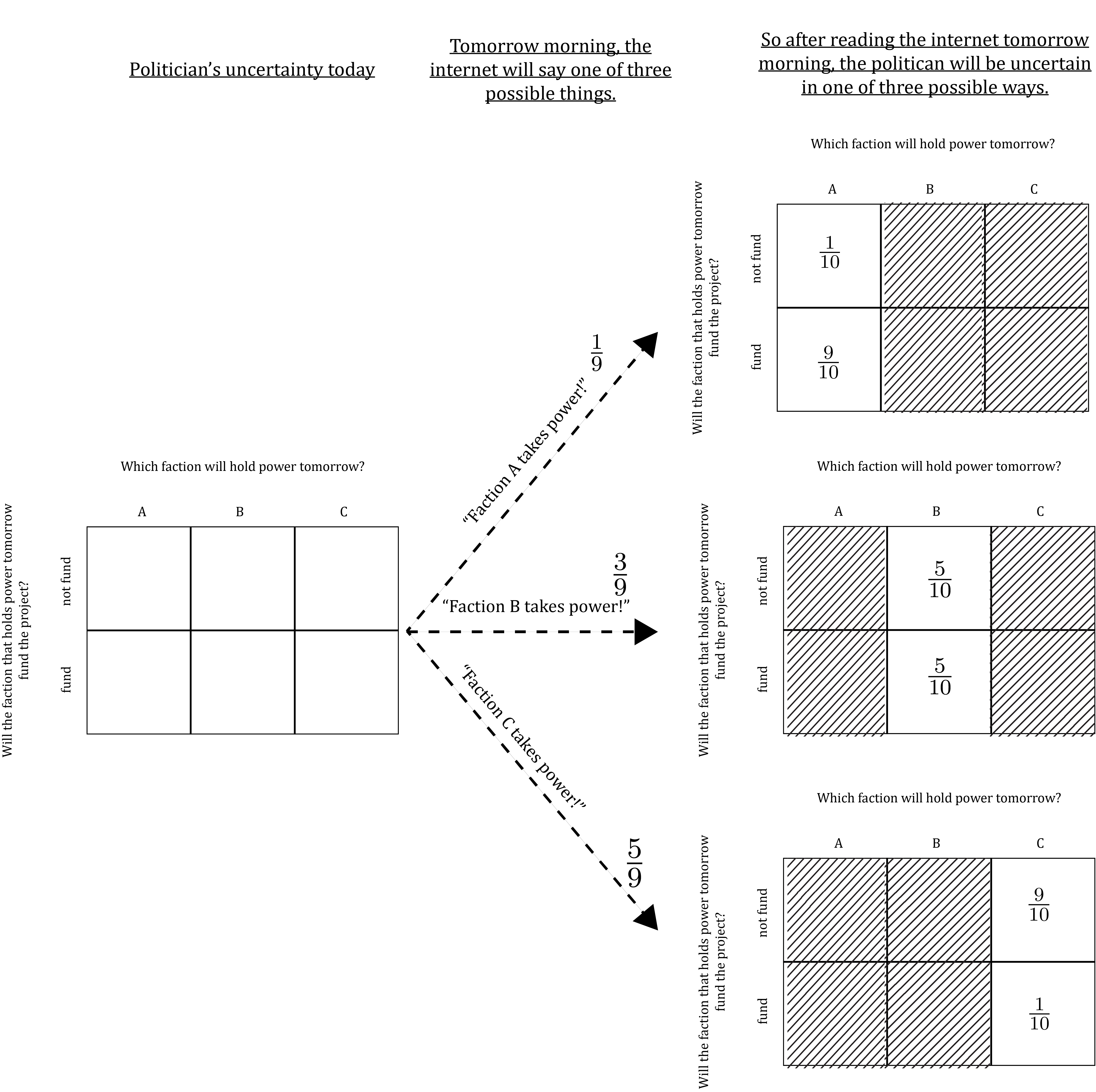
…then all of the joint probabilities are exactly determined as:
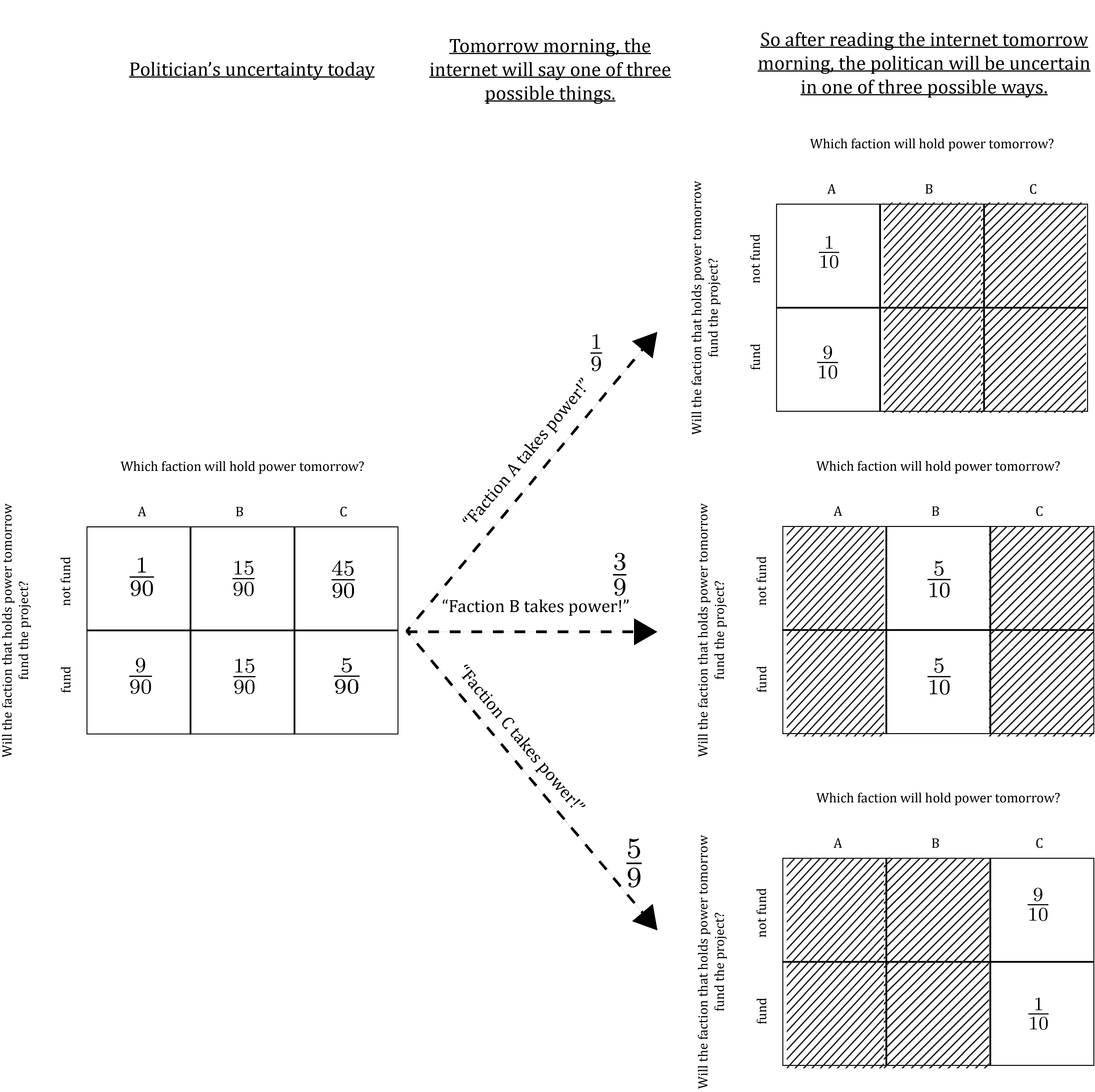
For instance, P(\text{fund \& $C$}) = P(C)P(\text{fund} | C). So, by setting P(C) = \frac{5}{9} and P(\text{fund} | C) = \frac{1}{10}, P(\text{fund \& $C$}) is fully determined as P(\text{fund \& $C$}) = \frac{5}{9} \times \frac{1}{10} = \frac{5}{90}
Conditional probability is especially useful for modeling interdependencies between multiple uncertainties. For instance, suppose we want to model the idea that A is most likely to fund the project if it takes power, B is somewhat less likely to fund the project if it takes power, and C is least likely to fund the project if it takes power. We can depict this idea by setting the conditional probabilities P(\text{fund} | A), P(\text{fund}| B) and P(\text{fund}| C) to values such that P(\text{fund} | A) > P(\text{fund} | B) > P(\text{fund} | C) For instance, here is a model of the politician’s uncertainty in which we assign values for the probabilities such that A is most likely to fund project, B is less likely and C is least likely:
Here’s a summary of the basic concepts in this section:
Pause and complete check of understanding 6 now!
The Marginal-Conditional Method for Modeling Joint Uncertainty
Because marginal and conditional probabilities together determine joint probabilities, you have two options when you want to build a probabilistic model depicting joint uncertainty. First, you can assign values to the joint probabilities in the model directly. Second, you can use what we’ll call the marginal-conditional method for modeling joint uncertainty. In practice, political scientists almost always use the marginal-conditional method.
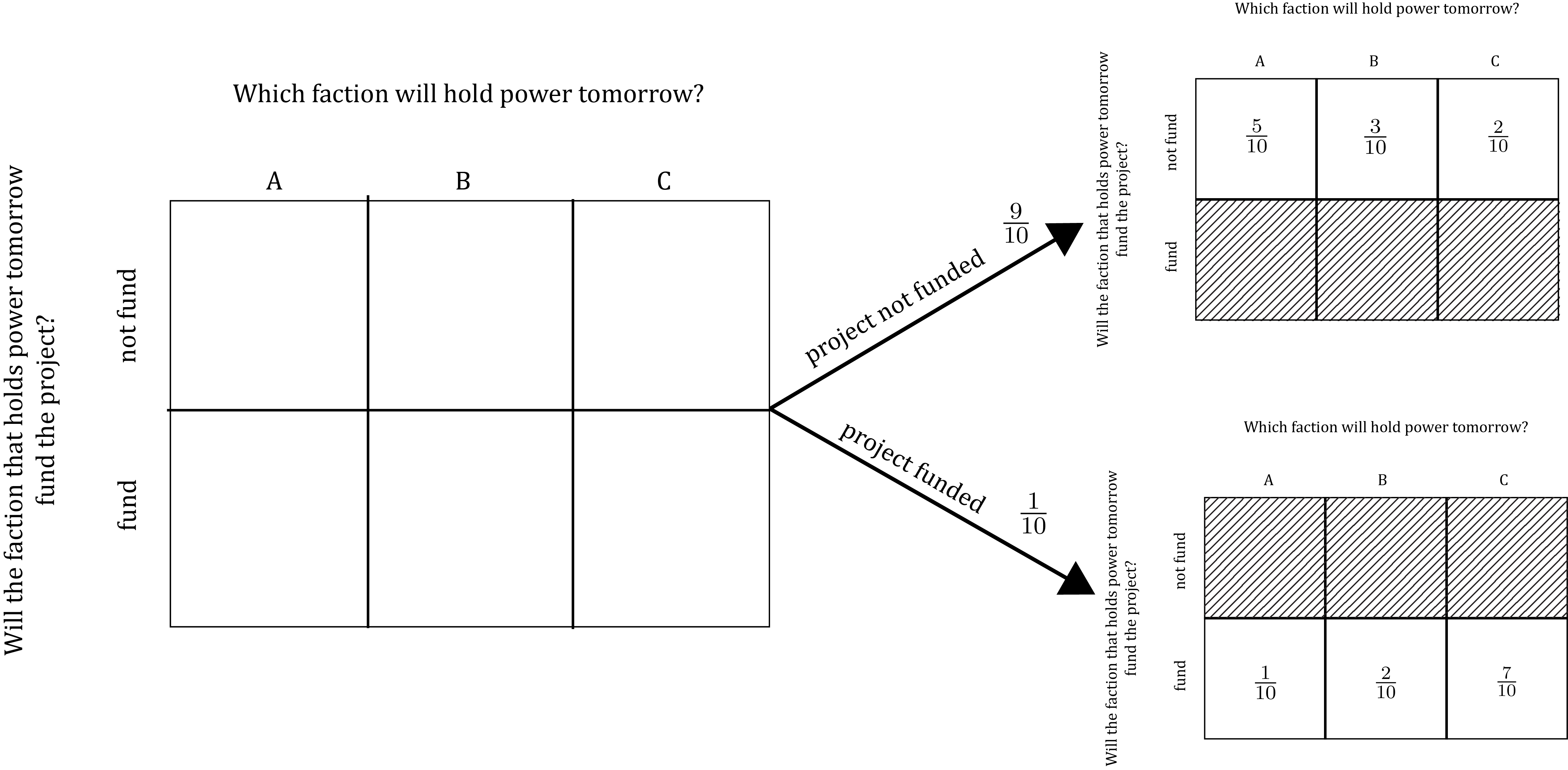
For example, consider the politician’s joint uncertainty about which faction will hold power tomorrow and whether the faction in power will fund the infrastructure project started today. Here’s how we would model this joint uncertainty using the marginal-conditional method:
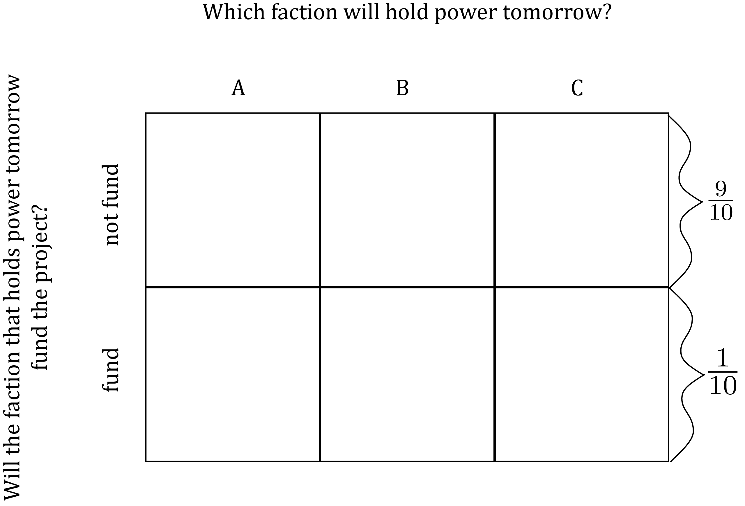
Step 1 – Model the marginal uncertainty about one of the two uncertainties. For instance, let’s model the marginal uncertainty about whether whichever faction holds power tomorrow will fund the project. This amounts to assigning values for the marginal probabilities P(\text{not fund}) and P(\text{fund}) that together sum to 1. For instance, suppose we want to depict the idea that the project is very unlikely to be funded, and so we set P(\text{not fund}) = \frac{9}{10} and P(\text{fund}) = \frac{1}{10} like this:
Step 2 – Model the other uncertainty conditional on each possible resolution of the uncertainty modeled in Step 1. Since we modeled uncertainty about whether the project will be funded in Step 1, this step involves modeling uncertainty about which faction will hold power conditional on whether the project is funded. Since there are two possible resolutions of the marginal uncertainty about whether the project will be funded – i.e. fund and not fund –, we need to model two different conditional uncertainties in this step. Specifically:
- Uncertainty about which faction will hold power conditional on the knowledge that the project will be funded.
- Uncertainty about which faction will hold power conditional on the knowledge that the project will not be funded.
In effect, this amounts to assigning conditional probabilities in each of the following models of conditional uncertainty:
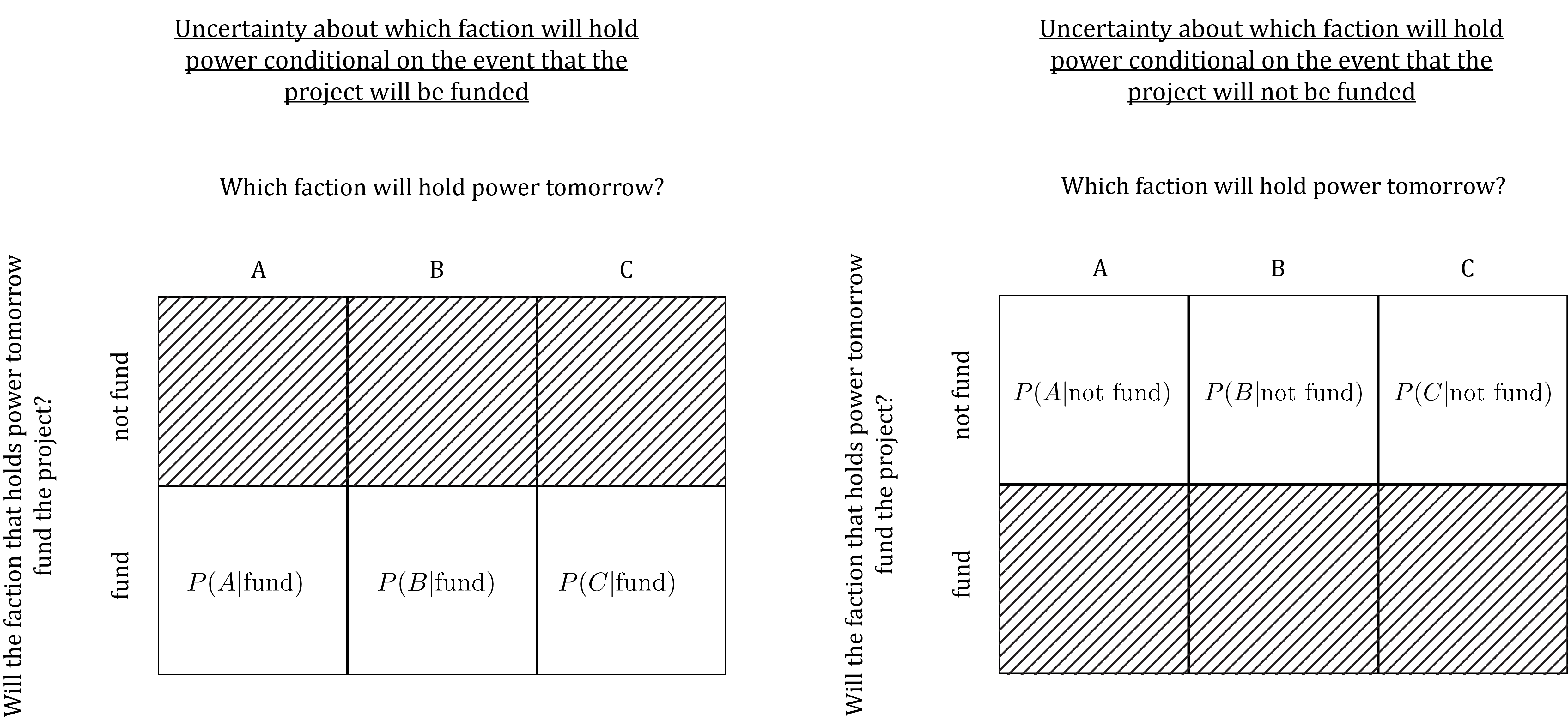
The probabilities we assign in this step are key for depicting interdependence between the uncertainties we want to model. For instance, suppose we want to model the idea that (1) if the project is funded, faction C is most likely to be in power, faction B is less likely, and faction A is least likely and (2) if the project is not funded, A is most likely to be in power, B less likely and C least likely. Then we would want to set the conditional probabilities in these models to values such that P(C|\text{fund}) > P(B|\text{fund}) > P(A|\text{fund}) and P(C|\text{not fund}) < P(B|\text{not fund}) < P(A|\text{fund}) For instance:
Step 3 – Compute the joint probabilities from the marginal and conditional probabilities. Having assigned marginal and conditional probabilities in Steps 1 and 2, you can now apply the identity P(X \& Y) = P(X)P(Y|X) = P(Y)P(X|Y) to determine the joint probabilities. For instance, above we set P(\text{fund}) = \frac{1}{10} and P(A | \text{fund}) = \frac{1}{10}, so the identity implies that P(A \& \text{fund}) = \frac{1}{10} \times \frac{1}{10} = \frac{1}{100}. More generally, the values we set in Steps 1 and 2 fully determine all the joint probabilities as follows:
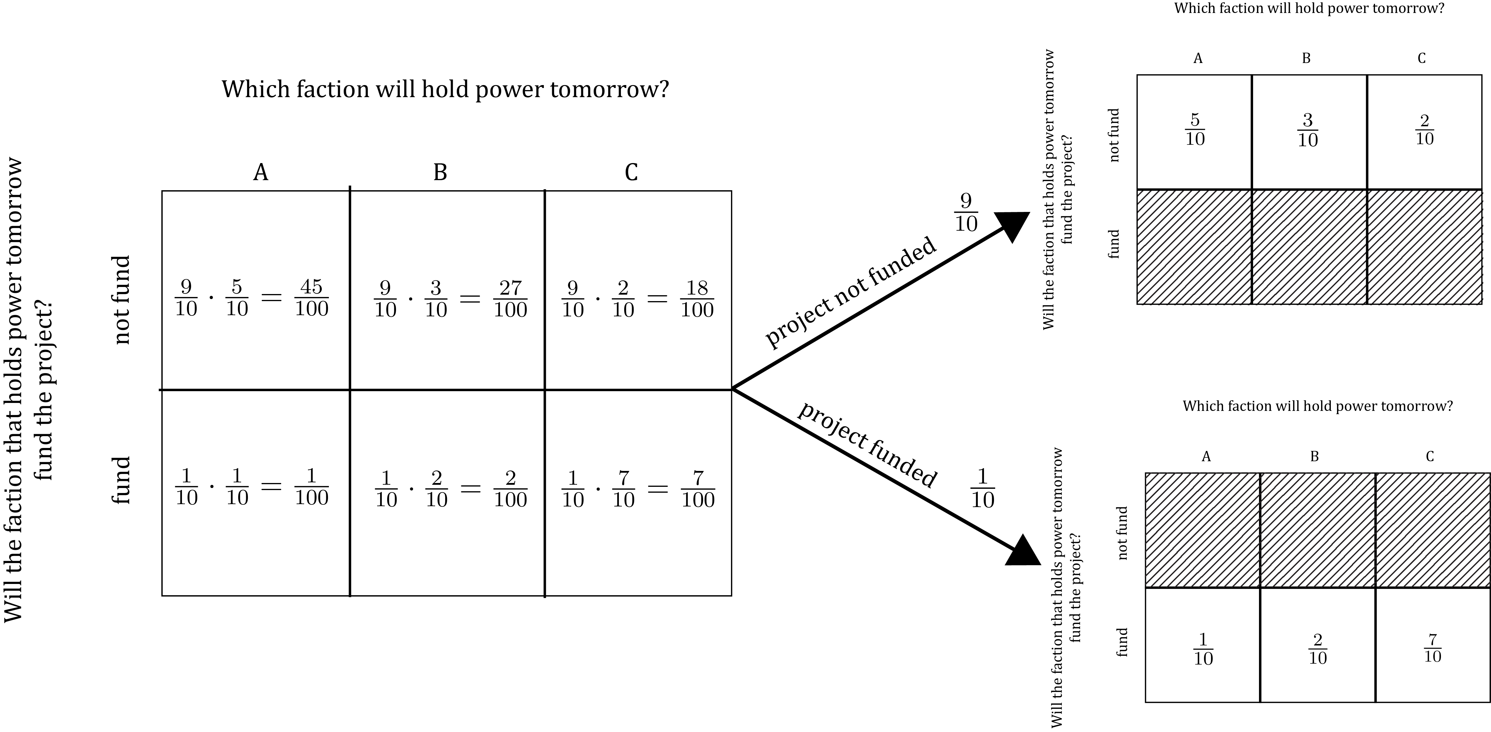
Pause and complete check of understanding 7 now!
Marginal-Conditional Diagrams
When we use the marginal-conditional method to build a model of multiple uncertainties, we often find that we need to use the marginal and conditional probabilities we specify to derive the values of additional probabilities. It’s always possible to work out these derivations using the formulas stated in this lesson that connect joint, marginal, and conditional probabilities. But relying on formulas is error-prone and can obscure the meaning of the derivations and their results. So in this section, you’ll learn a graphical represenatation of a probabilistic model specified using the marginal-conditional method called a Marginal-Conditional Diagram. You’ll then learn to use Marginal-Conditional Diagrams to calculate probabilities in ways that illustrate the meaning behind the calculations.
To illustrate, consider again the model we built in the previous section using the Marginal-Conditional Method:
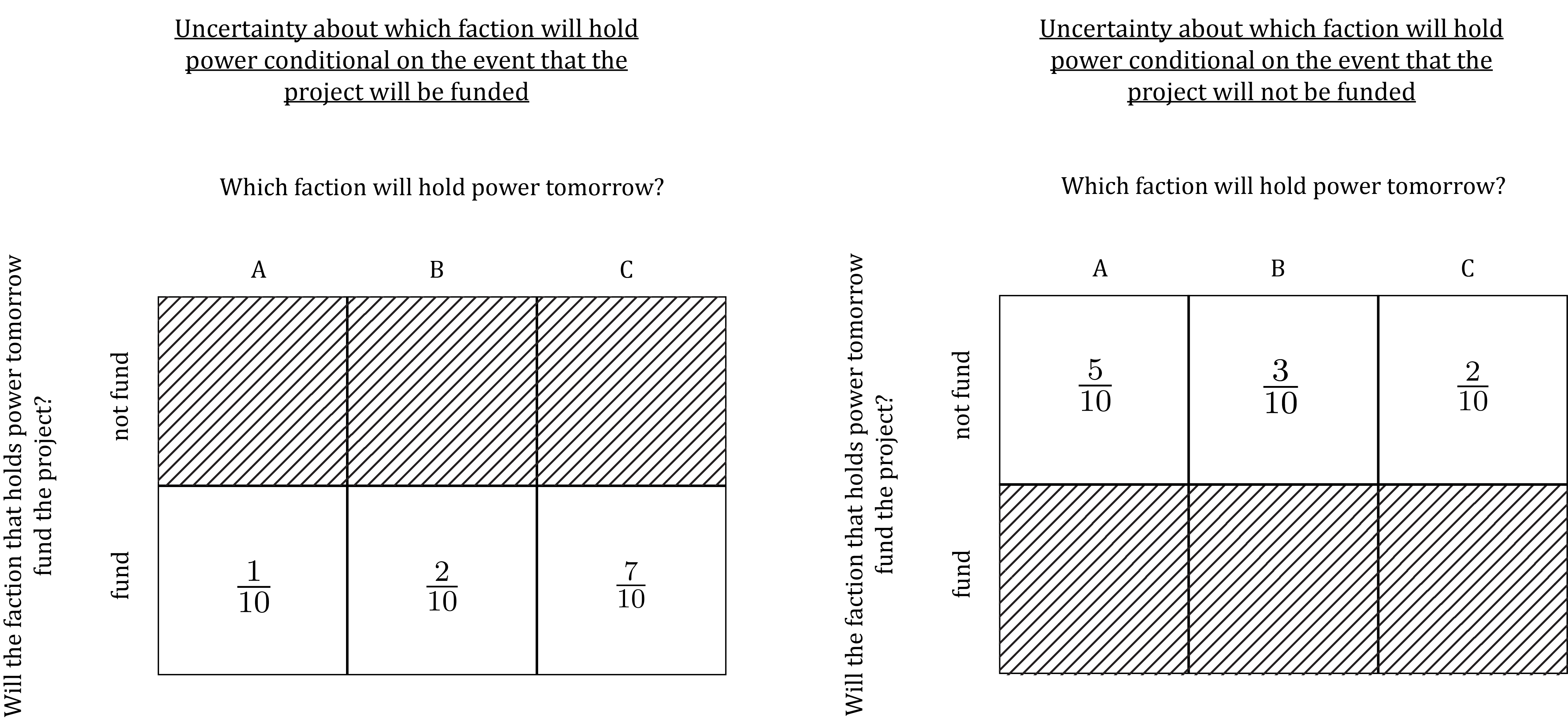
This model depicts the marginal uncertainty about whether the project will be funded like this:
| Event | Marginal Probability |
|---|---|
| project not funded | P(\text{not funded}) = \frac{9}{10} |
| project funded | P(\text{funded}) = \frac{1}{10} |
And it depicts the uncertainty about which faction will hold power conditional on whether the project is funded like this:
Conditional on the event that the project is not funded:
| Event | Conditional Probability |
|---|---|
| faction A holds power | P(A | \text{not funded}) = \frac{5}{10} |
| faction B holds power | P(B | \text{not funded}) = \frac{3}{10} |
| faction C holds power | P(C | \text{not funded}) = \frac{2}{10} |
Conditional on the event that the project is funded:
| Event | Conditional Probability |
|---|---|
| faction A holds power | P(A | \text{funded}) = \frac{1}{10} |
| faction B holds power | P(B | \text{funded}) = \frac{2}{10} |
| faction C holds power | P(C | \text{funded}) = \frac{7}{10} |
You’ve already seen how we can compute the joint probabilities in this model from the marginal and conditional probabilities. Specifically, we can directly apply the identity P(X \& Y) = P(X)P(Y|X) = P(Y)P(X|Y) For instance, since we posited that the marginal probability that project is funded is \frac{1}{10} and the probability that faction B takes power conditional on the project being funded is \frac{2}{10}, we can calculate the joint probability that the project is funded and B takes power like this: P(\text{$B$ \& funded}) = P(\text{funded})P(B|\text{funded}) = \frac{1}{10}\frac{2}{10} = \frac{2}{100}
But other probabilities in the model are a more complicated to derive. For instance, what if we want to derive the probability that the project will be funded conditional on the event that faction B takes power – i.e. the probability P(\text{funded} | B):
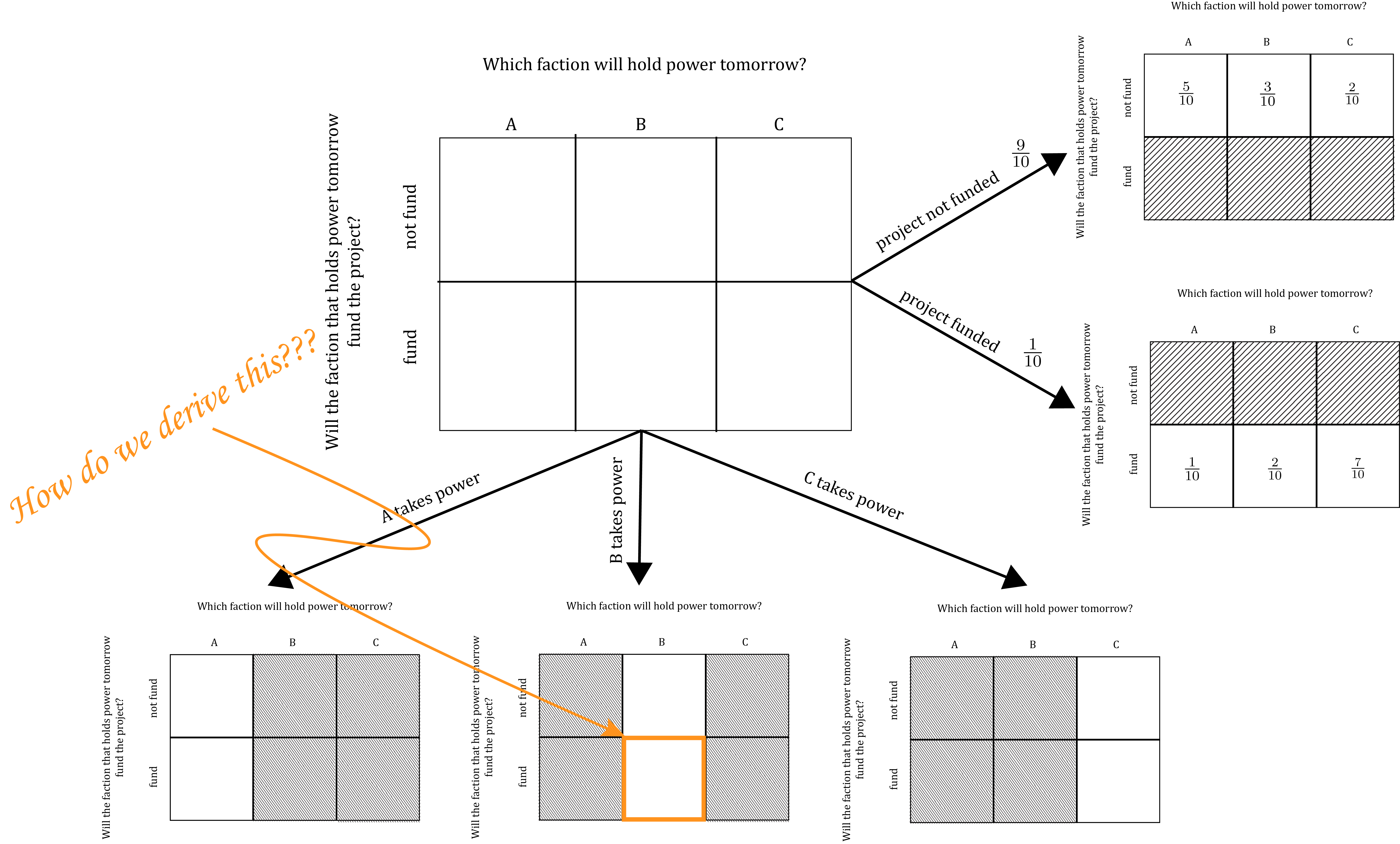
It turns out that applying all the formulas we’ve introduced so far, we can show that \begin{align*} P(\text{funded} | B) &= \frac{ P(\text{funded})P(B|\text{funded}) }{ P(\text{funded})P(B|\text{funded}) + P(\text{not funded})P(B|\text{not funded}) } \\\\ &= \frac{\frac{1}{10}\frac{2}{10}}{\frac{1}{10}\frac{2}{10} + \frac{9}{10}\frac{3}{10}} \\\\ &= \frac{2}{29} \end{align*} But figuring this out when you’re first learning the formulas that connection joint, marginal, and conditional probabilities is a lot of work that does little to develop your understanding of the logic and meaning of what you’re doing.
So, instead of learning to apply formulas to derive probabilities, you’ll use a graphical device that we’ll call a Marginal-Conditional Diagram. Learn how to build Marginal-Conditional Diagrams and use them to compute probabilities by watching the two videos linked below and completing the last two checks-of-understanding for this lesson:
Pause and complete check of understanding 8 now!
Pause and complete check of understanding 9 now!
Footnotes
A more realistic model would capture the fact that any level of flooding above the river’s normal level up to some maximum is possible. For instance, it might assume that the river could flood to any level between 0 and 3 meters above normal. A probabilistic model like that, in which the set of possible events amounts to all numbers between two limits, is called a “continuous” probability model. In contrast, a model in which the set of events can be described a list of distinct items, such as the levels 0, 1, 1.5, 2, 2.5, 3, is called a “discrete” probability model. Although discrete models can be simplistic, the analysis of continuous models requires knowledge of calculus. Thus these lessons will only use discrete models.↩︎
Calculations based on Bright Line Watch, 2022, “Bright Line Watch Survey Wave 17 Dataset”. https://brightlinewatch.org/survey-data-and-replication-material/↩︎