Lesson 6: Expected Utility

A natural event – a coastal storm, an earthquake, a forest fire – that becomes a human disaster of mass death, destruction and displacement renders a clear judgement on the past: Government should have done more to protect persons and their livelihoods from the coming hazard. That judgement, however, is retrospective. After the disaster, there is no uncertainty about the time, place or magnitude of the storm, earthquake or fire that wreaked havoc. We know – again, in retrospect, after the disaster – exactly what investments, whether in infrastructure, environmental conservation, economic regulation or the movement of populations, would have averted the tragedy.

But investments in resilience to environmental instability and change cannot, of course, be made in retrospect. By definition, the measures we take to mitigate the harms of natural hazards are taken prospectively. They are, therefore, decisions made under uncertainty. We cannot know, when we spend funds to enhance our infrastructure, or when we constrain how or how much we use our natural and economic resources, whether the measures we take will be adequate to the hazards of the future.

In modeling uncertainty thus far, we have focused on depicting the beliefs of political actors and how those beliefs might change in response to new information. In this lesson, we’ll progress to modeling decisionmaking under uncertainty – i.e. situations in which an actor must choose between actions that each have uncertain effects on outcomes. You’ll learn the standard tool used in PPT for modeling these choices, called expected utility.

Essential Features of Expected Utility Models

Every expected utility model has four elements:

Required Elements of an Expected Utility Model

Available Actions

A set of available actions between which a decisionmaker must choose.

Possible Outcomes

A set of possible outcomes that can result from any action chosen by the decisionmaker.

Conditional Probability Distributions

A set of conditional probability distributions, one distribution for each of the decisionmaker’s available actions. The distribution associated with a given action describes the relatively likelihood with which each possible outcome happens, given that the decisionmaker takes that action.

Utility Function

A utility function that assigns a utility level for the decisionmaker to each possible outcome.

We’ll illustrate each of these required elements by once again (hopefully you’re not too sick of this example by now!) imagining a city sitting on the bank of a flood prone river.

Suppose the mayor of the city is trying to decide whether to spend public funds to enhance the city’s flood control infrastructure. Specifically, she has two available actions:

Enhance the city’s flood control infrastructure.
Do not enhance the city’s flood control infrastructure.

In choosing between these actions, the mayor considers two competing priorities. On the one hand, when a storm comes up the river that is strong enough to overwhelm the city’s infrastructure, the city floods and the city’s residents suffer terribly. By enhancing it, the mayor can make the city’s infrastructure robust to stronger storms, and thus make floods of the city less likely. On the other hand, infrastructure enhancements sufficient to increase the city’s resilience to storms will require spending a large amount of scarce public funds, thereby neglecting other pressing public needs and weakening the mayor’s political support among some constituencies. Thus, the outcomes of the mayor’s choice that matter to her are (a) whether any future storm floods the city and (b) whether public funds are spent on infrastructure instead of other public needs. More specifically, the action the mayor takes will result in one of four possible outcomes:

The city does not flood and funds are spent on infrastructure instead of other public needs.
The city does not flood and funds are not spent on infrastructure instead of other public needs.
The city floods and funds are spent on infrastructure instead of other public needs.
The city floods and funds are not spent on infrastructure instead of other public needs.

Unfortunately, protecting cities from hurricanes and cyclones is an imperfect art. Thus by enhancing the city’s infrastructure, the mayor can reduce the likelihood that a storm will flood the city, but not eliminate uncertainty about whether the city will be flooded. Specifically, any one of three kinds of coastal storms can come up the mouth of the river and menace the city:

A weak storm to which the city’s current infrastructure is adequate just as it is. If this type of storm hits, the city will not flood regardless of whether the mayor has enhanced the city’s infrastructure.
A moderate storm that will overwhelm the city’s current infrastructure as it is but that will not overwhelm the enhanced infrastructure the mayor is considering. If this type of storm hits, the city will flood if the mayor has not enhanced the city’s infrastructure, and the city will not flood if the mayor has enhanced the city’s infrastructure.
A strong storm that will overwhelm both the city’s current infrastructure and the enhanced infrastructure the mayor is considering. If this type of storm hits, the city will flood regardless of whether the mayor has enhanced the city’s infrastructure.

We’ll begin by assigning specific numerical probabilities to each type of storm. Later in the lesson, once you’re familiar with the basic structure and analysis of expected utility models, we’ll explore a parameterized version of the model. Suppose that these three types of storms occur with the following probabilities:

Strength of Storm	Probability
weak	\frac{4}{9}
moderate	\frac{1}{3}
strong	\frac{2}{9}

Notice that the concept of conditional probability is key to depicting the implications of the mayor’s choice. Specifically, the probability distribution describing the likelihood the city will flood is conditional on which of her available actions the mayor chooses. Specifically, if the mayor does not enhance the city’s infrastructure, then the city floods if a moderate or strong storm hits the city. The marginal probability of either a moderate or strong storm hitting the city is \frac{2}{9} + \frac{1}{3} = \frac{5}{9}. On the other hand, if the mayor enhances the city’s infrastructure, then the city floods only if a strong storm hits the city, which occurs with probability \frac{2}{9}. We can thus describe the consequences of the mayor’s action with the following conditional probability distributions:

**If Mayor Does Not Enhance the City’s Infrastructure:**
Outcome	Probability
city floods and funds not spent on infrastructure	\frac{5}{9}
city does not flood and funds not spent on infrastructure	\frac{4}{9}

**If Mayor Enhances the City’s Infrastructure:**
Outcome	Probability
city floods and funds spent on infrastructure	\frac{2}{9}
city does not flood and funds spent on infrastructure	\frac{7}{9}

We now turn to depicting how the mayor values the city’s resilience to coastal storms relative to the other public needs she would have to neglect in order to enhance the city’s infrastructure. Before getting into the details, it’s critical to recognize a feature of this model that – like all expected utility models – distinguishes it from those used in Lesson 3 to illustrate utility representations of preference. The models in Lesson 3 depicted persons who were completely certain about the consequences of their actions for the priorities they cared about. In contrast, the mayor in this model is uncertain about whether either of her available courses of action will lead to her city being flooded. More specifically, this model draws a sharp distinction between the mayor’s available actions on the one hand, and the outcomes of those actions on the other. In models of choice under uncertainty, actions are the alternatives between which a decisionmaker has the power to choose. Outcomes, on the other hand, are the consequences that the decisionmaker cares about, which are only partially determined by the decisionmaker’s choice of action.

To keep the distinction clear between the things an actor has the ability to control (her actions) and the consequences of those actions (outcomes), expected utility models assign utility levels to each of the model’s possible outcomes, not to the available actions. Just as in the utility models of Lesson 3, a utility level is a number. The utility levels assigned to the outcomes are ordered to reflect the decisionmaker’s preference ordering over the outcomes, and the sizes of the gaps between the numbers depict the extent to which a gain or loss in one priority can be made up for by a loss or gain on another priority.

We’ll assign utility levels to outcomes in our model of the mayor’s decision in a way that emphasizes the tradeoff the mayor faces between the priority of preventing floods of the city, on the one hand, and the priority of spending funds on public needs other than infrastructure, on the other. To do this, we use a utility function that makes the interaction of these competing priorities explicit, by separating the mayor’s utility level into a “Benefit Term” and a “Cost Term”. Specifically, we’ll assign a utility level to each outcome given by:

\begin{array}{ccc} \undergroup{ \begin{Bmatrix} 1 & \text{if the city does not flood} \\ 0 & \text{if the city floods} \end{Bmatrix}} & - & \undergroup{ \begin{Bmatrix} \frac{1}{10} & \text{if funds ARE spent on infrastructure} \\ 0 & \text{if funds are ARE NOT spent on infrastructure} \end{Bmatrix}} \\ \text{Benefit Term} & & \text{Cost Term} \end{array}

Thus the mayor’s utility levels from each of the possible outcomes are:

Outcome	Mayor’s Utility Level
City does not flood and funds are spent on infrastructure	1-\frac{1}{10}
City does not flood and funds are not spent on infrastructure	1-0
City floods and funds are spent on infrastructure.	0-\frac{1}{10}
City floods and funds are not spent on infrastructure.	0-0

We’ve now specified all the elements required of an expected utility model. Here’s a summary:

An Expected Utility Model of Investments in Flood Control

Available Actions

The mayor can either enhance the city’s flood control infrastructure or not enhance the city’s flood control infrastructure.

Possible Outcomes

The city does not flood and funds are spent on infrastructure instead of other public needs.
The city does not flood and funds are not spent on infrastructure instead of other public needs.
The city floods and funds are spent on infrastructure instead of other public needs.
The city floods and funds are not spent on infrastructure instead of other public needs.

Distributions over Outcomes

**If Mayor Does Not Enhance the City’s Infrastructure:**
Outcome	Probability
city floods and funds not spent on infrastructure	\frac{5}{9}
city does not flood and funds not spent on infrastructure	\frac{4}{9}

**If Mayor Enhances the City’s Infrastructure:**
Outcome	Probability
city floods and funds spent on infrastructure	\frac{2}{9}
city does not flood and funds spent on infrastructure	\frac{7}{9}

Utility Function

Pause and complete check of understanding 1 now!

Pause and complete check of understanding 2 now!

Expected Utility

Imagine the mayor could somehow be given a guarantee that if she spends public funds to enhance the city’s infrastructure, the city will not flood with absolutely certainty; And if instead she refuses to spend funds to enhance the city’s infrastructure, the city will flood with certainty. Look again at the utility function we used to depict the mayor’s preferences over the model’s outcomes…

…and notice that it implies that the mayor’s utility level from spending the funds and avoiding a flood with certainty is 1-\frac{1}{10}=\frac{9}{10}, while her utility level from not spending the funds and having the city flooded with certainty is 0-0 = 0. So, in the model as we’ve specified it, the mayor would happily spend the money to enhance the city’s infrastructure if doing so would avert a flood with certainty.

For better or worse, however, the mayor has no available action that if taken will fully and completely determine whether the city floods. All that she is actually empowered to choose is the relative likelihood with which the city floods. In effect, by choosing whether or not to enhance the city’s infrastructure, the mayor chooses between two alternative probability distributions over the city’s possible flooding:

**If Mayor Does Not Enhance the City’s Infrastructure:**
Outcome	Probability
city floods and funds not spent on infrastructure	\frac{5}{9}
city does not flood and funds not spent on infrastructure	\frac{4}{9}

**If Mayor Enhances the City’s Infrastructure:**
Outcome	Probability
city floods and funds spent on infrastructure	\frac{2}{9}
city does not flood and funds spent on infrastructure	\frac{7}{9}

This is the nature of decisionmaking under uncertainty. When we choose under uncertainty, we do not get to directly select from the outcomes we care about. Instead, we choose between alternative probability distributions over those outcomes. Thus to depict a choice by the mayor between her actually available actions, we need a way to depict her preferences over probability distributions across outcomes, rather than over the outcomes themselves.

In PPT, expected utility is a method for assigning numerical values to probability distributions over outcomes that imply a preference ranking over those distributions. To understand expected utility, it helps to first understand the concept of a random variable.

Random Variable

A random variable is a set of possible numerical values along with a probability distribution describing the relative likelihoods of those values.

For instance:

Examples of Random Variables

Rolling a six-sided die

The number of pips on the face of a six-sided die that show up when the die is rolled is a random variable with the following probability distribution over its values:

Value	Probability
1	\frac{1}{6}
2	\frac{1}{6}
3	\frac{1}{6}
4	\frac{1}{6}
5	\frac{1}{6}
6	\frac{1}{6}

Number of students showing up to class

Imagine a college course in which 10 students are enrolled. Suppose that on any given day, the number of those 10 students who show up to class is a random variable with the following distribution:

Value	Probability
0	\frac{1}{100}
1	\frac{2}{100}
2	\frac{3}{100}
3	\frac{4}{100}
4	\frac{5}{100}
5	\frac{10}{100}
6	\frac{15}{100}
7	\frac{20}{100}
8	\frac{20}{100}
9	\frac{15}{100}
10	\frac{5}{100}

Hurricane categories

The Saffir-Simpson scale classifies hurricanes on a 1-5 scale on the basis of their wind speeds. By counting the number of hurricanes occuring in each category in each year, one could estimate the probability with which any given hurricane will be assigned one of the points on the scale. Thus, one could represent the Saffir-Simpson score of any given hurricane as a random variable like this:

Value	Probability
1	0.75
2	0.15
3	0.05
4	0.04
5	0.01

(To be clear, the probabilities above are made up, not based on actual hurricane data!)

The expected value of a random variable is a number that summarizes the variable’s distribution. Specifically:

Expected Value

Take any random variable with some number N values v_1, v_2, \ldots, v_N, which occur with probabilities p_1, p_2, \ldots, p_N, like so:

Value	Probability
v_1	p_1
v_2	p_2
\vdots	\vdots
v_N	p_N

The expected value (also called the mean value) of that random variable is given by:

v_1 \times p_1 + v_2 \times p_2 + \cdots + v_n \times p_N

Examples of Expected Values of Random Variables

Expected value of a six-sided die

The number of pips on the face of a six-sided die that show up when the die is rolled is a random variable with the following probability distribution over its values:

Value	Probability
1	\frac{1}{6}
2	\frac{1}{6}
3	\frac{1}{6}
4	\frac{1}{6}
5	\frac{1}{6}
6	\frac{1}{6}

Its expected value is:

1 \times \frac{1}{6} + 2 \times \frac{1}{6} + 3 \times \frac{1}{6} + 4 \times \frac{1}{6} + 5 \times \frac{1}{6} + 6 \times \frac{1}{6} = \frac{21}{6}

Number of students showing up to class

Imagine a college course in which 10 students are enrolled. Suppose that on any given day, the number of those 10 students who show up to class is a random variable with the following distribution:

Value	Probability
0	\frac{1}{100}
1	\frac{2}{100}
2	\frac{3}{100}
3	\frac{4}{100}
4	\frac{5}{100}
5	\frac{10}{100}
6	\frac{15}{100}
7	\frac{20}{100}
8	\frac{20}{100}
9	\frac{15}{100}
10	\frac{5}{100}

Its expected value is: \begin{equation*} \left( \begin{split} & 0 \times \frac{1}{100} + 1 \times \frac{2}{100} + 2 \times \frac{3}{100} +\\ & 3 \times \frac{4}{100} + 4 \times \frac{5}{100} + 5 \times \frac{10}{100} +\\ & 6 \times \frac{15}{100} + 7 \times \frac{20}{100} + 8 \times \frac{20}{100} + \\ & 9 \times \frac{15}{100} + 10 \times \frac{5}{100} \end{split} \right) = 6.65 \end{equation*}

Hurricane categories

The Saffir-Simpson scale classifies hurricanes on a 1-5 scale on the basis of their wind speeds. By counting the number of hurricanes occurring in each category in each year, one could estimate the probability with which any given hurricane will be assigned one of the points on the scale. Thus, one could represent the Saffir-Simpson score of any given hurricane as a random variable like this:

Value	Probability
1	0.75
2	0.15
3	0.05
4	0.04
5	0.01

Its expected value would be: 1 \times 0.75 + 2 \times 0.15 + 3 \times 0.05 + 4 \times 0.04 + 5 \times 0.01 = 1.41

In an expected utility model, a utility function assigns a utility level to each of the outcomes that can result from the decisionmaker’s chosen action. Thus, conditional on the action selected by the decisionmaker, the decisionmaker’s utility level is a random variable. For instance, in our model of the mayor’s choice, the probability distributions over the outcomes resulting from the mayor’s action are:

**If Mayor Does Not Enhance the City’s Infrastructure:**
Event	Probability
city floods and funds not spent	\frac{5}{9}
city does not flood and funds not spent	\frac{4}{9}

**If Mayor Enhances the City’s Infrastructure:**
Event	Probability
city floods and funds spent	\frac{2}{9}
city does not flood and funds spent	\frac{7}{9}

Applying the mayor’s utility function to these outcomes…

…we have that the mayor’s utility level is a random variable distributed conditional on her action as follows:

**If Mayor Does Not Enhance the City’s Infrastructure:**
Utility Level	Probability
0-0	\frac{5}{9}
1-0	\frac{4}{9}

**If Mayor Enhances the City’s Infrastructure:**
Utility Level	Probability
0-\frac{1}{10}	\frac{2}{9}
1-\frac{1}{10}	\frac{7}{9}

Computing the expected values of these random variables, then, yields the expected utilities to the mayor of each of her available actions:

Action	Expected Utility
Do not enhance infrastructure	[0-0] \times \frac{5}{9} + [1-0] \times \frac{4}{9} = \frac{4}{9}
Enhance infrastructure	\left[0-\frac{1}{10}\right] \times \frac{2}{9} + \left[1-\frac{1}{10}\right] \times \frac{7}{9} = \frac{61}{90}

In this model, then, the mayor receives higher expected utility from enhancing the city’s infrastructure than from not enhancing the city’s infrastructure.

Pause and complete check of understanding 3 now!

Pause and complete check of understanding 4 now!

Parameterized Models of Expected Utility

Expected utility models offer a relatively complex image of decisionmaking, in which choices depend on two distinct aspects of a situation: Beliefs about how choices affect the relative likelihoods of outcomes, on the one hand, and preferences over outcomes, on the other. Parameterized expected utility models allows us to depict the effects of each of these separate factors on choice.

In the model of the mayor’s choice between enhancing and not enhancing the city’s flood control infrastructure, the effects of the mayor’s action on the distribution of outcomes rests on an assumption about the likelihood of three types of storm:

A weak storm to which the city’s current infrastructure is adequate just as it is. If this type of storm hits, the city will not flood regardless of whether the mayor has enhanced the city’s infrastructure.
A moderate storm that will overwhelm the city’s current infrastructure as it is but that will not overwhelm the enhanced infrastructure the mayor is considering. If this type of storm hits, the city will flood if the mayor has not enhanced the city’s infrastructure, and the city will not flood if the mayor has enhanced the city’s infrastructure.
A strong storm that will overwhelm both the city’s current infrastructure and the enhanced infrastructure the mayor is considering. If this type of storm hits, the city will flood regardless of whether the mayor has enhanced the city’s infrastructure.

Suppose that the probabilities of the types of storm depend on a parameter \delta (the Greek letter pronounced “del-tah”) as follows:

Strength of Storm	Probability
weak	\frac{3}{4}(1-\delta)
moderate	\delta
strong	\frac{1}{4}(1-\delta)

Assume that the number \delta lies between 0 and 1. Under this assumption, weak storms are always three times more likely than strong storms, while moderate storms can range from extremely rare (when \delta is close to 0) to the vast majority of storms (when \delta is close to 1).

You can get a sense of how the distribution of storms varies with \delta by using this slider to set the value of \delta…

viewof delta = Inputs.range([0, 1], {value: 0.25, step: 0.01})

…and seeing how the relative likelihoods of the three kinds of storm respond:

{
  let levels = [
    {
      level: "weak",
      prob: 0.75*(1-delta)
    },
    {
      level: "moderate",
      prob: delta
    },
    {
      level: "strong",
      prob: 0.25*(1-delta)
    },
  ]
  let p = Plot.plot({
    marginTop: 10,
    marginRight: 30,
    marginBottom: 100,
    marginLeft: 100,
    width: width,
    height: 600,
    x: {domain: [0,1], label: 'Probability', labelAnchor: 'center', labelArrow: 'none'},
    y: {domain: ["strong", "moderate", "weak"], label: 'Strength of storm', labelAnchor: 'center', tickRotate: -90},
    marks: [
      Plot.barX(levels, {x: 'prob', y: 'level', fill: 'lightblue'}),
      Plot.text(levels, {x: 'prob', y: 'level', text: (d) => (d.prob).toFixed(2), dx: 20, fontSize: 30})
    ]
  })
  d3.select(p).selectAll("svg > g[aria-label='x-axis'] > text").style('font-size', '40px')
  d3.select(p).selectAll("svg > g[aria-label='y-axis'] > text").style('font-size', '40px')
  d3.select(p).selectAll("svg > g[aria-label='x-axis'] > g.tick > text").style('font-size', '20px')
  d3.select(p).selectAll("svg > g[aria-label='y-axis'] > g.tick > text").style('font-size', '30px')
  return p
}

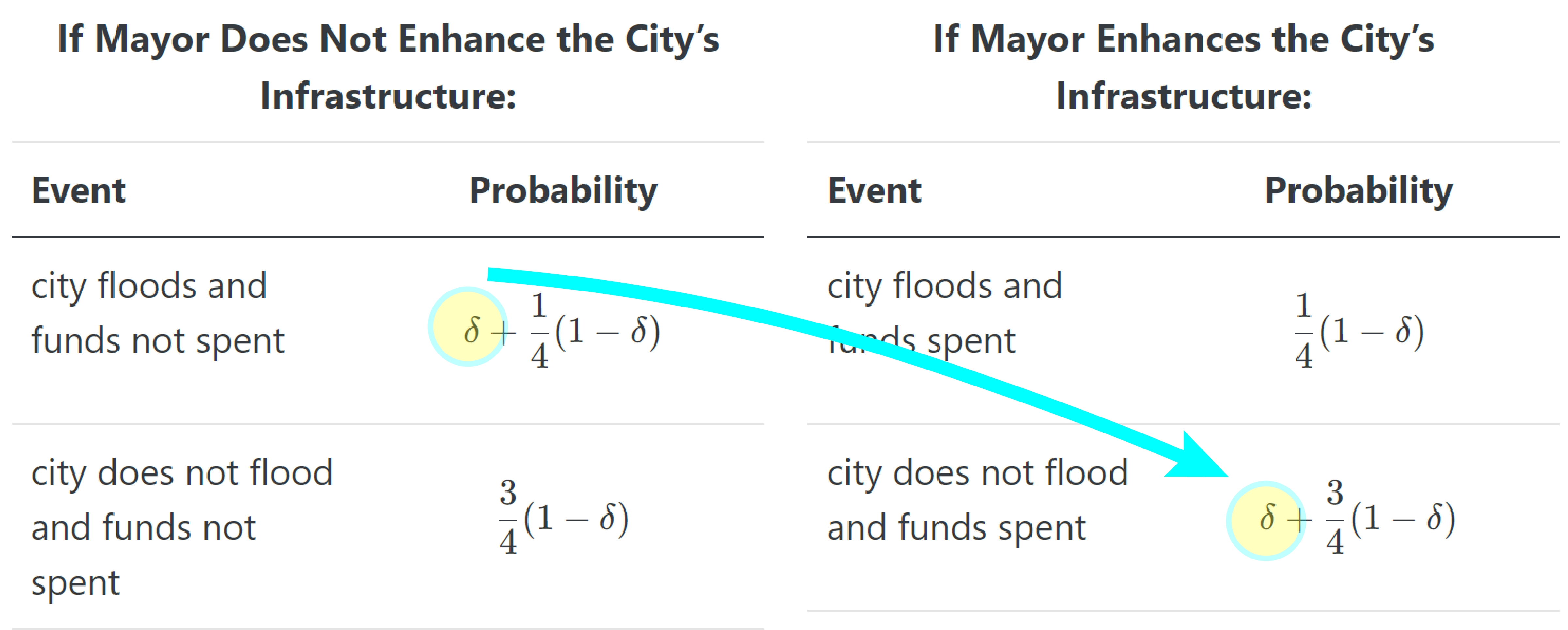
When storms are distributed as above, the effect of the mayor’s actions on the distribution of outcomes are given as:

**If Mayor Does Not Enhance the City’s Infrastructure:**
Event	Probability
city floods and funds not spent	\delta + \frac{1}{4}(1-\delta)
city does not flood and funds not spent	\frac{3}{4}(1-\delta)

**If Mayor Enhances the City’s Infrastructure:**
Event	Probability
city floods and funds spent	\frac{1}{4}(1-\delta)
city does not flood and funds spent	\delta + \frac{3}{4}(1-\delta)

Notice how parameterizing the distribution in this way reveals an essential structural feature of this model. By enhancing rather than not enhancing the city’s infrastructure, the mayor reduces the probability of a flood by a given amount (\delta) and increases the probability of no flood by that same amount. It looks like this:

Visually, you can see how the parameter \delta shifts the magnitude of the effect of the mayor’s choice on the probability of a flood by selecting a value for \delta using the following slider…

viewof deltaFlood = Inputs.range([0, 1], {value: 0.25, step: 0.01})

…and observing the resulting likelihoods that the city will flood conditional on the mayor’s action:

If Mayor Does Not Enhance Infrastructure

{
  let outcomes = [
    {
      outcome: "no flood",
      prob: 0.75*(1-deltaFlood)
    },
    {
      outcome: "flood",
      prob: deltaFlood + 0.25*(1-deltaFlood)
    }
  ]
  let p = Plot.plot({
    marginTop: 10,
    marginRight: 10,
    marginBottom: 60,
    marginLeft: 80,
    height: 500,
    x: {domain: [0,1], label: 'Probability', labelAnchor: 'center', labelArrow: 'none', grid: true},
    y: {domain: ["flood", "no flood"], label: 'Outcome', labelAnchor: 'center', tickRotate: -90},
    marks: [
      Plot.barX(outcomes, {x: 'prob', y: 'outcome', fill: 'lightblue'}),
      Plot.text(outcomes, {x: 'prob', y: 'outcome', text: (d) => (d.prob).toFixed(2), dx: 20, fontSize: 14}),
      Plot.ruleX([0])
    ]
  })
  d3.select(p).selectAll("svg > g[aria-label='x-axis'] > text").style('font-size', '20px')
  d3.select(p).selectAll("svg > g[aria-label='y-axis'] > text").style('font-size', '20px')
  d3.select(p).selectAll("svg > g[aria-label='y-axis'] > g.tick > text").style('font-size', '20px')
  return p
}

If Mayor Enhances Infrastructure

{
  let outcomes = [
    {
      outcome: "no flood",
      prob: deltaFlood + 0.75*(1-deltaFlood)
    },
    {
      outcome: "flood",
      prob: 0.25*(1-deltaFlood)
    }
  ]
  let p = Plot.plot({
    marginTop: 10,
    marginRight: 10,
    marginBottom: 60,
    marginLeft: 80,
    height: 500,
    x: {domain: [0,1], label: 'Probability', labelAnchor: 'center', labelArrow: 'none', grid: true},
    y: {domain: ["flood", "no flood"], label: 'Outcome', labelAnchor: 'center', tickRotate: -90},
    marks: [
      Plot.barX(outcomes, {x: 'prob', y: 'outcome', fill: 'lightblue'}),
      Plot.text(outcomes, {x: 'prob', y: 'outcome', text: (d) => (d.prob).toFixed(2), dx: 20, fontSize: 14})
    ]
  })
  d3.select(p).selectAll("svg > g[aria-label='x-axis'] > text").style('font-size', '20px')
  d3.select(p).selectAll("svg > g[aria-label='y-axis'] > text").style('font-size', '20px')
  d3.select(p).selectAll("svg > g[aria-label='y-axis'] > g.tick > text").style('font-size', '20px')
  return p
}

Play with the visualization above, and notice how the decrease in the probability of a flood caused by the mayor enhancing the city’s infrastructure varies with \delta. When \delta is small (i.e. close to 0), enhancing the city’s infrastructure only decreases the probability of a flood by a tiny amount. When \delta is large (i.e. close to 1), enhancing the city’s infrastructure causes a huge change in the likelihood of a flood.

How, then, does the parameter \delta impact the mayor’s willingness to enhance the city’s infrastructure? Recall once again he mayor’s utility function:

Applying this function to the distributions over outcomes induced by the mayor’s choice of action, we have the the mayor’s utility level is a random variable with the distributions:

**If Mayor Does Not Enhance the City’s Infrastructure:**
Utility Level	Probability
0-0	\delta + \frac{1}{4}(1-\delta)
1-0	\frac{3}{4}(1-\delta)

**If Mayor Enhances the City’s Infrastructure:**
Utility Level	Probability
0-\frac{1}{10}	\frac{1}{4}(1-\delta)
1-\frac{1}{10}	\delta + \frac{3}{4}(1-\delta)

Thus the mayor’s expected utility from each of her available actions is:

Action	Expected Utility
Do not enhance infrastructure	[1-0]\frac{3}{4}(1-\delta) + [0-0]\left[ \delta + \frac{1}{4}(1-\delta) \right]
enhance infrastructure	\left[1-\frac{1}{10}\right]\left[\delta + \frac{3}{4}(1-\delta)\right] + \left[0-\frac{1}{10}\right]\left[ \frac{1}{4}(1-\delta) \right]

The expressions for the mayor’s expected utility each have a common structure. Making this structure clear clarifies the role of the parameter \delta in the mayor’s incentives. First observe that for each of her actions, the expression for the mayor’s expected utility has the form:

\left[\text{\large benefit of a flood} - \text{\large cost term}\right]\left[ \text{\large probability of a flood} \right] + \left[\text{\large benefit of no flood} - \text{\large cost term}\right]\left[ \text{\large probability of no flood} \right]

Now observe that for each of the mayor’s actions, the cost term is the same regardless of whether the city floods. Specifically, the cost term is 0 if the mayor does not enhance the city’s infrastructure and \frac{1}{10} if the mayor does the city’s infrastructure. Thus we can re-write the expression for the mayor’s expected utility as:

\begin{equation*} \begin{split} & \left[\text{\large benefit of a flood}\right]\left[ \text{\large probability of a flood} \right] + \left[\text{\large benefit of no flood}\right]\left[ \text{\large probability of no flood} \right] \\ & - \left[\text{\large cost term}\right]\left[ \text{\large probability of a flood} + \text{\large probability of no flood} \right] \end{split} \end{equation*}

Now note that conditional on the mayor’s action, \text{\large probability of a flood} + \text{\large probability of no flood} = 1 Thus the expression for the mayor’s expected utility from either action can be simplified to:

\left[\text{\large benefit of a flood}\right]\left[ \text{\large probability of a flood} \right] + \left[\text{\large benefit of no flood}\right]\left[ \text{\large probability of no flood} \right] - \left[\text{\large cost term}\right]

Further, the term “benefit of a flood” is equal to 0 in the mayor’s utility function, so the expression further simplifies as:

\left[\text{\large benefit of no flood}\right]\left[ \text{\large probability of no flood} \right] - \left[\text{\large cost term}\right]

Thus we can re-write the mayor’s expected utility from each of her actions as:

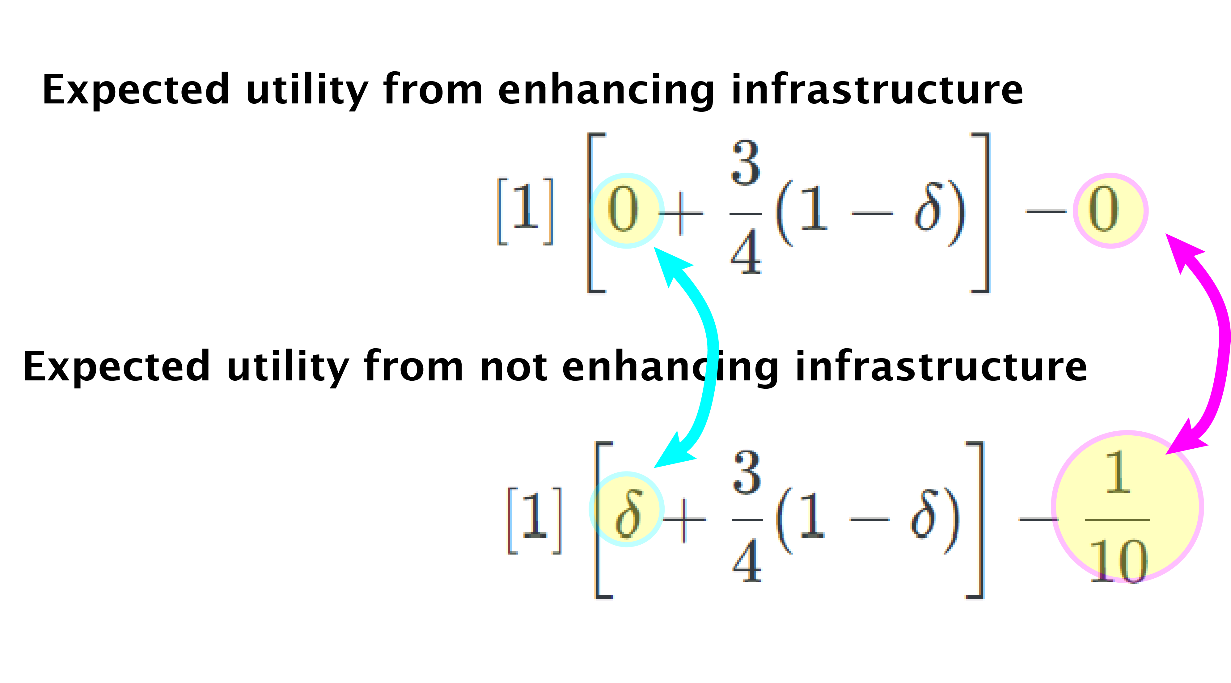
Action	Expected Utility
Do not enhance infrastructure	[1]\left[0+\frac{3}{4}(1-\delta)\right] - 0
enhance infrastructure	\left[1\right]\left[\delta + \frac{3}{4}(1-\delta)\right] -\frac{1}{10}

Written this way, we can see the precise nature of the tradeoff the mayor faces when she chooses whether to enhance the city’s infrastructure. By enhancing the city’s infrastructure, she increases the probability of no flood by \delta but does so by incurring a utility cost of \frac{1}{10}. It looks like this:

So, whether the mayor gets a higher expected utility from enhancing the city’s infrastructure depends on the the size of \delta – i.e. the probability of a ‘moderate’ storm – relative to the size the cost she pays for spending funds on infrastructure instead of other public needs. This means that she will tend to prefer to enhance the city’s infrastructure when the likelihood of a moderate storm (\delta) is high and she will prefer to not enhance the city’s infrastructure when the likelihood of a moderate storm is low.

You can see this pattern in operation by using the following slider to choose a value for \delta…

viewof deltaEU = Inputs.range([0, 1], {value: 0.25, step: 0.01})

…and observing the resulting expected utility levels from each of the mayor’s available actions:

{
  let actions = [
    {
      action: "do not enhance",
      eu: 0.75*(1-deltaEU)
    },
    {
      action: "enhance",
      eu: deltaEU + 0.75*(1-deltaEU) - 0.1
    }
  ]
  let p = Plot.plot({
    marginTop: 10,
    marginRight: 10,
    marginBottom: 60,
    marginLeft: 80,
    height: 500,
    x: {domain: [0,1], label: 'Expected Utility', labelAnchor: 'center', labelArrow: 'none', grid: true},
    y: {domain: ["do not enhance", "enhance"], label: 'Action', labelAnchor: 'center', tickRotate: -90},
    marks: [
      Plot.barX(actions, {x1: 0, x2: 'eu', y: 'action', fill: 'lightblue'})
    ]
  })
  d3.select(p).selectAll("svg > g[aria-label='x-axis'] > text").style('font-size', '20px')
  d3.select(p).selectAll("svg > g[aria-label='y-axis'] > text").style('font-size', '20px')
  d3.select(p).selectAll("svg > g[aria-label='y-axis'] > g.tick > text").style('font-size', '20px')
  return p
}

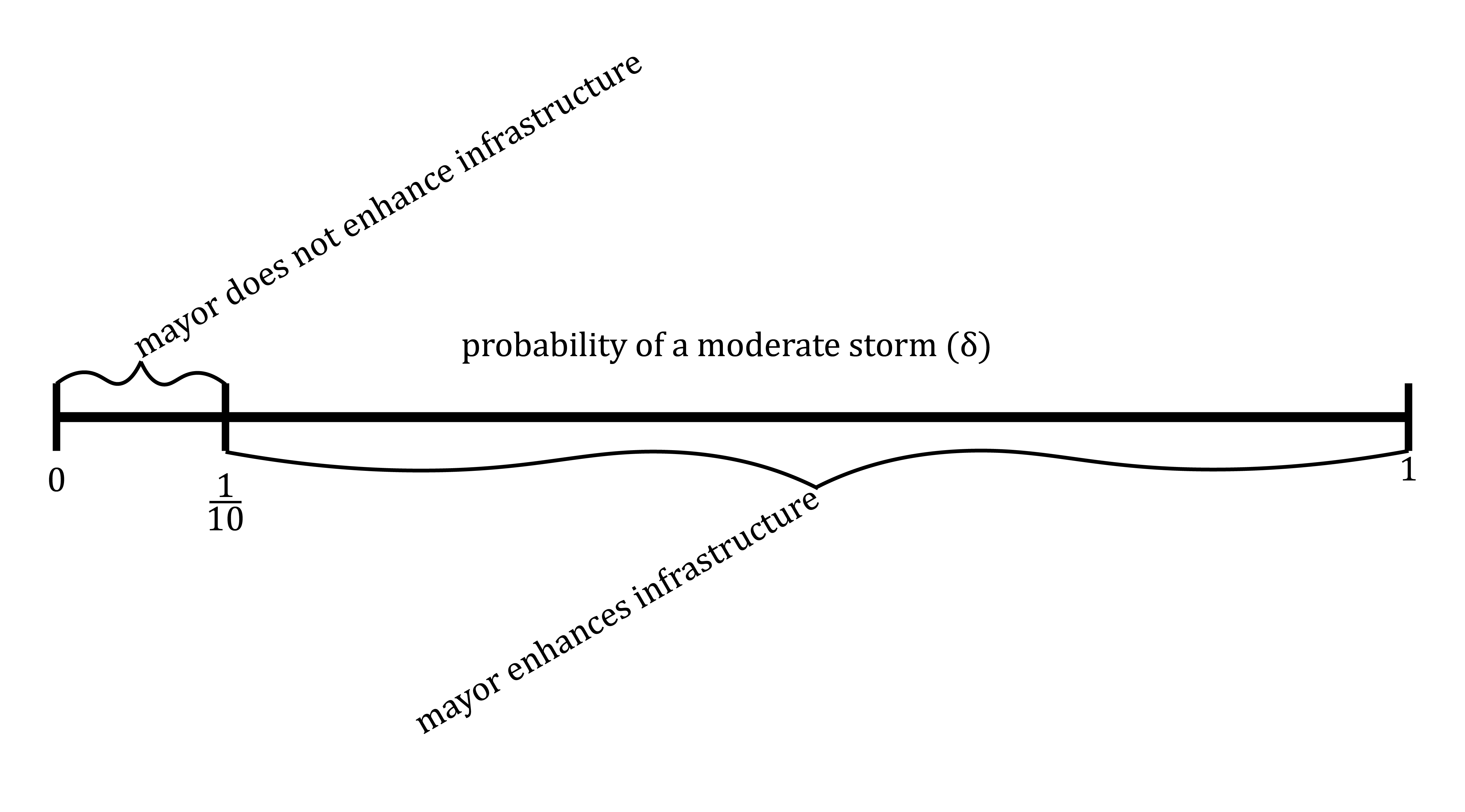
The key thing to observe as you play with the display above is that for small values of \delta (specifically, for \delta < \frac{1}{10}), the mayor’s expected utility from not enhancing the infrastructure is higher than from enhancing it. On then other hand for large values of \delta (specifically \delta > \frac{1}{10}), the mayor’s expected utility from not enhancing the infrastructure is lower than from enhancing it.

In effect, there is a “threshold implication” in this model. When \delta is above this threshold, the mayor will enhance the city’s flood control infrastructure and when \delta is below this threshold she won’t. To see this, write the inequality that must hold for the mayor’s expected utility from enhancing the city’s infrastructure to be higher than her expected utility from not enhancing the city’s infrastructure: \left[1\right]\left[\delta + \frac{3}{4}(1-\delta)\right] -\frac{1}{10} \geq \left[1\right]\left[ \frac{3}{4}(1-\delta)\right] -0 Subtracting \frac{3}{4}(1-\delta) from both sides and adding \frac{1}{10} to both sides, that inequality becomes: \delta \geq \frac{1}{10} So we can summarize the effect of the parameter \delta – i.e. the likelihood of a moderate storm – on the mayor’s incentives in a diagram like this:

To see another example of a parameterized expected utility model and its analysis, watch the video here:

Pause and complete check of understanding 5 now!